RecoTour III: Variational Autoencoders for Collaborative Filtering with Mxnet and Pytorch
A deep dive into the use of Variational Autoencoders for Collaborative Filtering


- 1. Variational Autoencoders for collaborative filtering
- 2. Preparing the data
- 3 $\text{Mult-VAE}^{\text{PR}}$: the code
- 4. Train, validate and test model
- 5. Summary of the results
This post and the code here are part of a larger repo called RecoTour, where I normally explore and implement some recommendation algorithms that I consider interesting and/or useful (see RecoTour and RecoTourII). In every directory, I have included a README file and a series of explanatory notebooks that I hope help explaining the code. I keep adding algorithms from time to time, so stay tunned if you are interested.
As always, let me first acknowledge the relevant people that did the hard work. This post and the companion repo are based on the papers “Variational Autoencoders for Collaborative Filtering” [1] and "Auto-Encoding Variational Bayes" [2]. The code here and in that repo is partially inspired by the implementation from Younggyo Seo. I have adapted the code to my coding preferences and added a number of options and flexibility to run multiple experiment.
The reason to take a deep dive into variational autoencoders for collaborative filtering is because they seem to be one of the few Deep Learning based algorithm (if not the only one) that is obtains better results that those using non-Deep Learning techniques [3].
All the experiments in this post were run using a p2.xlarge EC2 instance on AWS.
1. Variational Autoencoders for collaborative filtering
I must admit that when it comes to variational autoencoders (VAEs) I find that there is a "notable" difference between the complexity of the math and that of the code (or maybe is just me that I am not a mathematician). Nonetheless, I think that speaking about VAEs and not mentioning log likelihoods, Evidence Lower Bound (EBLO) or the Kullback–Leibler divergence ($\text{D}_{\text{KL}}$) is almost like "cheating". With that in mind I will try to give some mathematical context to "Partially Regularized Multinomial Variational Autoencoder" ($\text{Mult-VAE}^{\text{PR}}$) for collaborative filtering and then move to the code. The whole purpose of the math below is to ultimately justify the loss function we will be using when training the $\text{Mult-VAE}^{\text{PR}}$ as well as the architecture of the algorithm.
Before diving into the problem scenario and the mathematical formulation, let me describe the notational convention. Following Liang et al., 2018, I will use $u \in \{1,\dots,U\}$ to index users and $i \in \{1,\dots,I\}$ to index items. The user-by-item binary interaction matrix (i.e. the click matrix) is $\mathbf{X} \in \mathbb{N}^{U\times I}$ and I will use lower case $\mathbf{x}_u =[X_{u1},\dots,X_{uI}]^\top \in \mathbb{N}^I$ to refer to the click history of an individual user $u$.
1.1 Problem scenario
We are given a dataset $\mathbf{X} = \{ {\mathbf{x}_u} \}^{U}_{u=1}$ of user clicks (a more general scenario is described in "Auto-Encoding Variational Bayes" [2]). Our job is to estimate the parameters of the underlying probability distribution so that we can do inference. In other words, we need to find a statistical model of the data (like in any other ML problem). To do this, we need to maximize the likelihood function $p_{\theta}(\mathbf{X})$ so that under the assumed statistical model the observed data is most probable.
To find the maximum likelihood we could assume that the statistical model of the data involves some latent variable $\bf{z}$, so that the marginal likelihood can be written as:
$$ p_{\theta}(\mathbf{x}_u) = \int {p_{\theta}(\mathbf{z}_u)p_{\theta}(\mathbf{x}_u \vert \mathbf{z}_u) d\mathbf{z}_u} \hspace{1cm} (1) $$where $\theta$ are the parameters of the distribution. Eq (1) is solvable if we assume that both the prior $p_{\theta}(\mathbf{z}_u)$ and the conditional probability $p_{\theta}(\mathbf{x}_u \vert \mathbf{z}_u)$ come from parametric families of distributions and that their PDFs are differentiable almost everywhere w.r.t. both $\theta$ and $\mathbf{z}_u$. However, for "moderately" complicated likelihood functions $p_{\theta}(\mathbf{x}_u \vert \mathbf{z}_u)$, such as a neural network with a nonlinear layer, Eq (1) is intractable (it is not possible to evaluate of differentiate the marginal likelihood). Furthermore, the true posterior $p_{\theta}(\mathbf{z}_u \vert \mathbf{x}_u) = p_{\theta}(\mathbf{x}_u \vert \mathbf{z}_u)p_{\theta}(\mathbf{z}_u)/p_{\theta}(\mathbf{x}_u)$ is also intractable, and therefore we cannot use an EM algorithm (since the E-step involves the computation of the true posterior at a given iteration).
To address these and some other limitations, and find a general solution to this problem, Kingma and Welling 2014 proposed a flexible neural network based approach.
1.2 Auto-Encoding Variational Bayes
The following Section is both a summary and my understanding of the paper "Auto-Encoding Variational Bayes" to which I keep referring and that I strongly recommend reading.
Let me remind you: our goal is to maximize the likelihood, or more conveniently the log likelihood $\log p_{\theta}(\mathbf{X})$, where:
$$ \log p_{\theta}(\mathbf{X}) = \sum_u \log p_{\theta}(\mathbf{x}_u) \hspace{1cm} (2) $$Each term in the summation can be re-written as:
$$ \log p_{\theta}(\mathbf{x}_u) = D_{KL}\left(q_\phi(\textbf{z}_u\vert \textbf{x}_u) \| p_\theta(\textbf{z}_u \vert \textbf{x}_u)\right) + \underbrace{\mathbb{E} \small{ q_{\phi}(\mathbf{z}_u \vert \mathbf{x}_u) } \left[ -\log q_{\phi}(\mathbf{z}_u \vert \mathbf{x_u}) + \log p_{\theta}(\mathbf{x}_u, \mathbf{z}_u) \right]}_{ELBO \mathcal L(\textbf{x}_u, \phi,\theta)} \hspace{1cm} (3) $$Where the first elements in the right hand side is the Kullback–Leibler divergence ($\text{D}_{\text{KL}}$) and $q_\phi(\textbf{z}_u\vert \textbf{x}_u)$ is the approximate posterior of the true posterior $p_\theta(\textbf{z}_u \vert \textbf{x}_u)$. Eq (3) is our "point of entry" from which we will derive the remaining equations. If you want proof of Eq (3) I would recommend reading this tutorial or this "crazy" post.
Moving on, given that $\text{D}_{\text{KL}}$ is non-negative, $\log p_{\theta}(\mathbf{x}_u) \geq \mathcal L(\textbf{x}_u, \phi,\theta)$ and therefore $\mathcal L$ is referred as Evidence Lower Bound (ELBO). It is straightforward to understand from Eq (3) that maximizing $\log p_{\theta}(\mathbf{x}_u)$ implies maximizing ELBO $\mathcal L$. If we re-order the terms in that equation, we could also think of the problem as follows: maximizing ELBO $\mathcal L$ implies minimizing $\text{D}_{\text{KL}}$, which makes sense, since $D_{KL}$ measures the dissimilarity between the approximate posterior $q_\phi(\textbf{z}_u\vert \textbf{x}_u)$ and the true posterior $p_{\theta}(\textbf{z}_u\vert \textbf{x}_u)$.
ELBO $\mathcal L$ in Eq (3) can also be re-written as:
$$ \mathcal L(\textbf{x}_u, \phi,\theta) = - D_{KL}\left(q_\phi(\textbf{z}_u\vert \textbf{x}_u) \| p_\theta(\textbf{z}_u \right) + \mathbb{E} \small{ q_{\phi}(\mathbf{z}_u \vert \mathbf{x}_u) } \left[ \log p_{\theta}(\textbf{x}_u\vert \textbf{z}_u) \right] \hspace{1cm} (4) $$We can see that Eq (4) involves sampling $\tilde{\mathbf{z}_u} \sim q_{\phi}(\mathbf{z}_u \vert \mathbf{x}_u)$. When sampling is involved, backpropagation is not trivial (how one would take gradients with respect to $\phi$?). To remedy this situation Kingma & Welling introduced the so called "reparameterization trick". Instead of sampling from the approximate postertior $q_{\phi}(\mathbf{z}_u \vert \mathbf{x}_u)$, the authors used a differentiable transformation $g_{\phi}(\mathbf{\epsilon}, \mathbf{x}_u)$ of a noise variable $\epsilon$, such that:
$$ \tilde{\mathbf{z}_u} = g_{\phi}(\mathbf{\epsilon}, \mathbf{x}_u) \hspace{1cm} with \hspace{1cm} \mathbf{\epsilon} \sim p(\epsilon) \hspace{1cm} (5) $$where $p(\epsilon)$ can be, for example, a variable sampled from a random normal distribution (see Section 1.3 for the selection of $g_{\phi}$ in the particular case of the $\text{Mult-VAE}^{\text{PR}}$). With these formulation, one can use Monte Carlo estimates of expectations of some function $f(\mathbf{z})$ with respect to $q_{\phi}(\mathbf{z}_u \vert \mathbf{x}_u)$ such that:
$$ \mathbb{E} \small{ q_{\phi}(\mathbf{z}_u \vert \mathbf{x}_u) }\left[ f(\mathbf{z}_u) \right] = \mathbb{E} \small{ q_{\phi}(\mathbf{z}_u \vert \mathbf{x}_u) }\left[ f(g_{\phi}(\mathbf{\epsilon}, \mathbf{x}_u)) \right] \simeq \frac{1}{L} \sum_{l=1}^{L} f(g_{\phi}(\mathbf{\epsilon}^l), \mathbf{x}_u) \\ \text{where} \hspace{1cm} \mathbf{\epsilon}^l \sim p(\epsilon) \hspace{1cm} (6) $$Replacing the second term in Eq (4) with the result in Eq (6), we see that the ELBO $\mathcal L$ can be approximated by what Kingma and Welling called "Generic Stochastic Gradient Variational Bayes" (SGVB) estimator $\tilde{\mathcal L}(\textbf{x}_u, \phi,\theta) \simeq \mathcal L(\textbf{x}_u, \phi,\theta)$:
$$ \tilde{\mathcal L}(\mathbf{x}_u, \phi,\theta) = - D_{KL}\left(q_\phi(\textbf{z}_u\vert \textbf{x}_u) \| p_\theta(\textbf{z}_u \right) + \frac{1}{L} \sum_{l=1}^{L} \log p_{\theta}(\mathbf{x}_u \vert \mathbf{z}^l_u) \\ \text{where} \hspace{1cm} \mathbf{z}^l_u = g_{\phi}(\epsilon^l_u, \mathbf{x}_u) \hspace{1cm} \text{and} \hspace{1cm} \epsilon^l \sim p(\epsilon) \hspace{1cm} (7) $$Of course, when running a practical application, we will be using minibatches. With that in mind, we can re-write ELBO $\mathcal{L}$ in "minibatch form" as:
$$ \mathcal L(\mathbf{\text{X}}^M, \phi,\theta) \simeq \tilde{\mathcal L}^{M}(\mathbf{\text{X}}^M, \phi,\theta) = \frac{1}{M} \sum_{u=1}^{M} \tilde{\mathcal L}(\mathbf{x}_u, \phi,\theta) \hspace{1cm} (8) $$where $\mathbf{X}^M = \{\mathbf{x}_u \}_{u=1}^M$ is a minibatch of M users. In their experiments the authors found that the number of samples $L$ can be set to 1 as long as the minibatch size was large enough, e.g. $M$ = 100. Therefore, as long as our batch sizes are of 100 or more, Eq (7) can be re-written as:
$$ \mathcal L(\mathbf{\text{X}}^M, \phi,\theta) \simeq \frac{1}{M} \sum_{u=1}^{M} - D_{KL}\left(q_\phi(\textbf{z}_u\vert \textbf{x}_u) \| p_\theta(\textbf{z}_u \right) + \log p_{\theta}(\mathbf{x}_u \vert \mathbf{z}^s_u) \hspace{1cm} (9) $$Note that $\mathbf{z}^s_u$ signifies that $\mathbf{z}_u$ still needs to be sampled once from $q_\phi(\textbf{z}_u\vert \textbf{x}_u)$, but using the reparameterization trick this will be rather easy, as we will see in the next section. Finally, now that we have a "nice looking" mathematical expression, this is how Auto-Encoding Variational Bayes works:
- Select a prior for latent representation of $\textbf{x}_u$, $p_{\theta}(\textbf{z}_u)$
- Use a neural network to parameterize the distribution $p_{\theta}(\textbf{x}_u\vert \textbf{z}_u)$. Because this part of the model maps the latent variable/representation $\textbf{z}_u$ to the observed data $\textbf{x}_u$, it is referred as a "decoder" network.
- Rather than explicitly calculating the intractable posterior $p_{\theta}(\textbf{z}_u\vert \textbf{x}_u)$, use another another neural network to parameterize the distribution $q_\phi(\textbf{z}_u\vert \textbf{x}_u)$ as the approximate posterior. Since $q_\phi$ maps the observed data $\textbf{x}_u$ to the latent space of $\textbf{z}_u$'s, is referred as the "encoder" network.
- maxmize ELBO $\mathcal{L}$ in Eq (9) using Stochastic Gradient Descent or any of its cousins
1.3 Partially Regularized Autoencoder for Collaborative Filtering
or $\text{Mult-VAE}^{\text{PR}}$...
In the previous Section we obtained Eq (9), which is a generic form of the function we need to maximize to solve the problem described in Section 1.1. Now let's see a particular case of that equation for the set up used by Liang and co-authors in their paper. Such set up is described as follows: for each user $u$, the latent representation $\textbf{z}_u$ is assumed to be drawn from a standard Gaussian prior $p(\textbf{z}_u) \sim \mathcal N(0, I)$. Such representation is then transformed by a multi-layer perceptron (MLP), and the output is normalized via a Softmax function to produce a probability distribution over all items $I$, $\pi(\mathbf{z}_u) = Softmax(MLP(\mathbf{z}_u))$. Then, the click history of user $u$ is assumed to be drawn from a Multinomial distribution with probability $\pi(\mathbf{z}_u)$:
$$ \textbf{x}_u \sim \text{Mult}(N_u, \pi(\mathbf{z}_u)) \hspace{1cm} (10) $$where $N_u = \sum_i x_{ui}$ is the total number of clicks for user $u$. In this set up, the log-likelihood of the click history $\mathbf{x}_u$ conditioned to the latent representation $\mathbf{z}_u$ is simply:
$$ \begin{equation*} \log(p_{\theta}(\textbf{x}_u\vert \textbf{z}_u)) = \mathbf{x}_u \log(\pi(\mathbf{z}_u)) \hspace{1cm} (11) \end{equation*} $$The posterior $q_\phi(\textbf{z}_u\vert \textbf{x}_u)$ is also chosen to be a standard Gaussian $q_\phi(\textbf{z}_u\vert \textbf{x}_u) \sim \mathcal N(\mu_\phi(\textbf{x}_u), \sigma_\phi(\textbf{x}_u) I)$ where $\mu_\phi(\textbf{x}_u)$ and $\sigma_\phi(\textbf{x}_u)$ are functions implemented as neural networks. Then, we use the reparameterization trick and chose $g_{\phi}(\mathbf{\epsilon}, \mathbf{x}_u) = \mu(\textbf{x}_u) + \sigma(\textbf{x}_u) \cdot \epsilon$, where $\epsilon \sim \mathcal{N}(0,I)$. This way $\mathbf{z}^s_u = \mu(\textbf{x}_u) + \sigma(\textbf{x}_u) \cdot \epsilon$ where we sample directly $\epsilon$.
At this stage we have defined the Gaussian prior, the Gaussian approximate posterior and our sampled latent representation. We are finally ready to "plug the terms" into Eq (9) and write the loss function that we will minimize when training the Mult-VAE:
$$ Loss = -\frac{1}{M} \sum_{u=1}^{M} \left[ \mathbf{x}_u \log(\pi(\mathbf{z}_u)) + \frac{\beta}{2} \sum_j ( 1 + \log(\sigma_{uj}^2) - \mu_{uj}^2 - \sigma_{uj}^2 ) \right] \hspace{1cm} (12) $$Note that the expression above is the negative ELBO $\mathcal L$ (maximizing $\mathcal L$ is equivalent to minimize -$\mathcal L$) with a multiplicative factor $\beta$ applied to the $D_{KL}$. For the math behind the $D_{KL}$ expression given this set up have a look here.
Let me just comment on that $\beta$. Looking at the loss function in Eq (12) within the context of VAEs, we can see that the first term is the reconstruction loss, while the $D_{KL}$ act as a regularizer. With that in mind, Liang et al add a factor $\beta$ to control the strength of the regularization, and propose $\beta < 1$.
Let's pause for one second and think on what this means. First of all, we are no longer optimizing a lower bound for a given log likelihood. In addition, remember that the $D_{KL}$ divergence measures the similarity between the approximate posterior $q_\phi(\textbf{z}_u\vert \textbf{x}_u)$ and the prior $p_\theta(\textbf{z}_u)$. Therefore, by using $\beta < 1$ we are weakening the influence of the prior constrain $q_\phi(\textbf{z}_u\vert \textbf{x}_u) \approx p_\theta(\textbf{z}_u)$ on the loss. This means that we are less able to generalize to novel user clicks from historical data. However, when building recommendation systems we are often not interested in reproducing precisely click histories (i.e. achieving the best loss) but in making good recommendations (i.e. achieving the best ranking metrics). As the authors show in the paper (and we will see here later), the best ranking metrics are obtained when using $\beta < 1$ and in consequence they name the algorithm Partially Regularized Multinomial Autoencoder or $\text{Mult-VAE}^{\text{PR}}$.
2. Preparing the data
Throughout this exercise I will use two dataset. The Amazon Movies and TV dataset [4] [5] and the Movilens dataset. The later is used so I can make sure I am obtaining consistent results to those obtained in the paper. As we will see through the notebook, the Amazon dataset is significantly more challenging that the Movielens dataset.
The data preparation is fairly simple, and is identical for both datasets. Therefore, I will focus here only on the Amazon dataset.
#collapse-hide
import os
import sys
import pandas as pd
import numpy as np
import pickle

from tqdm import trange
from typing import Tuple, Dict, Union
from pathlib import Path

sys.path.append(os.path.abspath('/Users/javier/ml_experiments_python/RecoTour/Amazon/mult-vae/'))
rootpath = Path("/Users/javier/ml_experiments_python/RecoTour/Amazon/mult-vae/")
DATA_DIR = Path(rootpath / 'data')
new_colnames = ["user", "item", "rating", "timestamp"]

inp_path = DATA_DIR / "amazon-movies"
filename = "reviews_Movies_and_TV_5.p"
raw_data = pd.read_pickle(inp_path / filename)
keep_cols = ["reviewerID", "asin", "overall", "unixReviewTime"]
raw_data = raw_data[keep_cols]
raw_data.columns = new_colnames
print(raw_data.shape)
raw_data.head()
def get_count(tp: pd.DataFrame, id: str) -> pd.Index:
    """
    Returns `tp` groupby+count by `id`
    """
    playcount_groupbyid = tp[[id]].groupby(id, as_index=False)
    count = playcount_groupbyid.size()
    return count


def filter_triplets(
    tp: pd.DataFrame, min_user_click, min_item_click
) -> Tuple[pd.DataFrame, pd.Index, pd.Index]:
    """
    Returns triplets (`tp`) of user-item-rating for users/items with
    more than min_user_click/min_item_click counts
    """
    if min_item_click > 0:
        itemcount = get_count(tp, "item")
        tp = tp[tp["item"].isin(itemcount.index[itemcount >= min_item_click])]

    if min_user_click > 0:
        usercount = get_count(tp, "user")
        tp = tp[tp["user"].isin(usercount.index[usercount >= min_user_click])]

    usercount, itemcount = get_count(tp, "user"), get_count(tp, "item")

    return tp, usercount, itemcount
filtered_raw_data, user_activity, item_popularity = filter_triplets(
    raw_data, min_user_click=5, min_item_click=0
)
Note that, since I am using the "reviews_Movies_and_TV_5" (i.e. the 5-core dataset, where users and items have at least 5 reviews each) filtered_raw_data has no effect on the Amazon dataset. It does however filter some users/items in the case of the Movilens dataset.
Let's now have a look to the sparsity of the dataset:
sparsity = (
    1.0
    * filtered_raw_data.shape[0]
    / (user_activity.shape[0] * item_popularity.shape[0])
)

print(
    "After filtering, there are %d watching events from %d users and %d movies (sparsity: %.3f%%)"
    % (
        filtered_raw_data.shape[0],
        user_activity.shape[0],
        item_popularity.shape[0],
        sparsity * 100,
    )
)
Comparing these numbers to those of the Movilens dataset (9990682 watching events from 136677 users and 20720 movies: sparsity: 0.353%. see the notebook corresponding to the original publication, or the original publication itself) one can see that the Amazon dataset is $\sim$13 times more sparse than the Movielens dataset. In consequence, I one would expect that the algorithm finds it more challenging, resulting in lower ranking metrics.
def split_users(
    unique_uid: pd.Index, test_users_size: Union[float, int]
) -> Tuple[pd.Index, pd.Index, pd.Index]:

    n_users = unique_uid.size

    if isinstance(test_users_size, int):
        n_heldout_users = test_users_size
    else:
        n_heldout_users = int(test_users_size * n_users)

    tr_users = unique_uid[: (n_users - n_heldout_users * 2)]
    vd_users = unique_uid[(n_users - n_heldout_users * 2) : (n_users - n_heldout_users)]
    te_users = unique_uid[(n_users - n_heldout_users) :]

    return tr_users, vd_users, te_users
unique_uid = user_activity.index
np.random.seed(98765)
idx_perm = np.random.permutation(unique_uid.size)
unique_uid = unique_uid[idx_perm]
tr_users, vd_users, te_users = split_users(
    unique_uid, test_users_size=0.1
)
print(tr_users.shape, vd_users.shape, te_users.shape)
And this is how the authors set up the experiment: for validation and test they consider "only" items that have been seen during training
# Select the training observations raw data
tr_obsrv = filtered_raw_data.loc[filtered_raw_data["user"].isin(tr_users)]
tr_items = pd.unique(tr_obsrv["item"])

# Save index dictionaries to "numerise" later one
item2id = dict((sid, i) for (i, sid) in enumerate(tr_items))
user2id = dict((pid, i) for (i, pid) in enumerate(unique_uid))

vd_obsrv = filtered_raw_data[
    filtered_raw_data["user"].isin(vd_users)
    & filtered_raw_data["item"].isin(tr_items)
]

te_obsrv = filtered_raw_data[
    filtered_raw_data["user"].isin(te_users)
    & filtered_raw_data["item"].isin(tr_items)
]
Now that we have the validation and test users and their interactions, we will split such interactions into so-called "validation and test train and test sets".
I know that this sounds convoluted, but is not that complex. The "validation_train and test_train sets", comprising here 80% of the total validation and test sets, will be used to build what we could think as an input binary "image" (i.e. the binary matrix of clicks) to be "encoded -> decoded" by the trained auto-encoder. On the other hand the "validation_test and test_test sets", comprising here 20% of the total validation and test sets, will be used to compute the ranking metrics at validation/test time. If you want more details along with a toy example please go to the corresponding notebook in the repo. I will discuss this further in Section 4.
def split_train_test(
    data: pd.DataFrame, test_size: float
) -> Tuple[pd.DataFrame, pd.DataFrame]:

    data_grouped_by_user = data.groupby("user")
    tr_list, te_list = list(), list()

    np.random.seed(98765)

    for i, (nm, group) in enumerate(data_grouped_by_user):
        n_items_u = len(group)

        if n_items_u >= 5:
            idx = np.zeros(n_items_u, dtype="bool")
            idx[
                np.random.choice(
                    n_items_u, size=int(test_size * n_items_u), replace=False
                ).astype("int64")
            ] = True

            tr_list.append(group[np.logical_not(idx)])
            te_list.append(group[idx])
        else:
            tr_list.append(group)

    data_tr = pd.concat(tr_list)
    data_te = pd.concat(te_list)

    return data_tr, data_te


def numerize(tp: pd.DataFrame, user2id: Dict, item2id: Dict) -> pd.DataFrame:
    user = [user2id[x] for x in tp["user"]]
    item = [item2id[x] for x in tp["item"]]
    return pd.DataFrame(data={"user": user, "item": item}, columns=["user", "item"])
vd_items_tr, vd_items_te = split_train_test(vd_obsrv, test_size=0.2)
te_items_tr, te_items_te = split_train_test(te_obsrv, test_size=0.2)
And that's it regarding to data preparation. We can now move to the model itself.
3 $\text{Mult-VAE}^{\text{PR}}$: the code
After the explanation in Section 1 you might expect the code to look rather complex. However, you might feel disappointed/pleased when you see how simple it really is.
In the original publications the authors used a one hidden layer MLP as generative model. There they say that deeper architectures do not improve the results, which I find it to be true after having run over 60 experiments. With that it mind, let's first have a look the model $ I \rightarrow 600 \rightarrow 200 \rightarrow 600 \rightarrow I$, where $I$ is the total number of items:
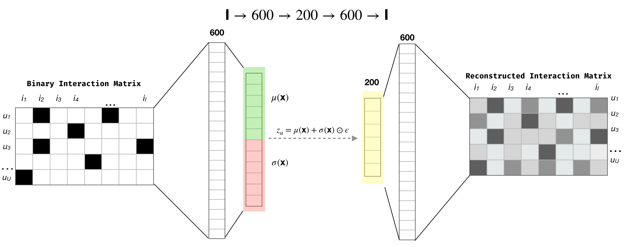
Figure 1. $\text{Mult-VAE}^{\text{PR}}$ architecture. The colors in the Figure are my attempt to emphasize the reparameterization trick.
In code, the figure above is:
#collapse-hide
from typing import List

import numpy as np

import mxnet as mx
from mxnet import autograd, gluon, nd
from mxnet.gluon import nn, HybridBlock
class VAEEncoder(HybridBlock):
    def __init__(self, q_dims: List[int], dropout: List[float]):
        super().__init__()

        # last dim multiplied by two for the reparameterization trick
        q_dims_ = q_dims[:-1] + [q_dims[-1] * 2]
        with self.name_scope():
            self.q_layers = nn.HybridSequential(prefix="q_net")
            for p, inp, out in zip(dropout, q_dims_[:-1], q_dims_[1:]):
                self.q_layers.add(nn.Dropout(p))
                self.q_layers.add(nn.Dense(in_units=inp, units=out))

    def hybrid_forward(self, F, X):
        h = F.L2Normalization(X)
        for i, layer in enumerate(self.q_layers):
            h = layer(h)
            if i != len(self.q_layers) - 1:
                h = F.tanh(h)
            else:
                mu, logvar = F.split(h, axis=1, num_outputs=2)
        return mu, logvar
class Decoder(HybridBlock):
    def __init__(self, p_dims: List[int], dropout: List[float]):
        super().__init__()

        with self.name_scope():
            self.p_layers = nn.HybridSequential(prefix="p_net")
            for p, inp, out in zip(dropout, p_dims[:-1], p_dims[1:]):
                self.p_layers.add(nn.Dropout(p))
                self.p_layers.add(nn.Dense(in_units=inp, units=out))

    def hybrid_forward(self, F, X):
        h = X
        for i, layer in enumerate(self.p_layers):
            h = layer(h)
            if i != len(self.p_layers) - 1:
                h = F.tanh(h)
        return h
class MultiVAE(HybridBlock):
    def __init__(
        self,
        p_dims: List[int],
        dropout_enc: List[float],
        dropout_dec: List[float],
        q_dims: List[int] = None,
    ):
        super().__init__()

        self.encode = VAEEncoder(q_dims, dropout_enc)
        self.decode = Decoder(p_dims, dropout_dec)

    def hybrid_forward(self, F, X):
        mu, logvar = self.encode(X)
        std = F.exp(0.5 * logvar)
        eps = F.random.normal_like(std)
        sampled_z = mu + float(autograd.is_training()) * eps * std
        return self.decode(sampled_z), mu, logvar
Before I move on, let me mention (and appreciate) one of the many nice "little" things that Mxnet's Gluon has to offer. You will notice the use of HybridBlock and the use of the input F (the backend) when we define the forward pass, or more precisely, the hybrid_forward pass. One could write a full post on the joys of HybridBlocks and how nicely and easily the guys that developed Gluon brought together the flexibility of imperative frameworks (e.g. Pytorch) and the speed of declarative frameworks (e.g. Tensorflow) together. If you want to learn the details go here, but believe me, this is FAST.
Having said that, there is only one more piece that we need to have the complete model, the loss function in Eq (12).
def vae_loss_fn(inp, out, mu, logvar, anneal):
    # firt term
    neg_ll = -nd.mean(nd.sum(nd.log_softmax(out) * inp, -1))
    # second term without beta
    KLD = -0.5 * nd.mean(nd.sum(1 + logvar - nd.power(mu, 2) - nd.exp(logvar), axis=1))
    # "full" loss (anneal is beta in the expressions above)
    return neg_ll + anneal * KLD
In the paper the authors also use a Multinomial Denoising Autoencoder (Mult-DAE). The architecture is identical to that of the $\text{Mult-VAE}^{\text{PR}}$ apart from the fact that there is no variational aspect. I have implemented the Mult-DAE and run multiple experiments with it. However, given its simplicity and an already lengthy post, I will not discuss the corresponding code here.
Let's have a look to the MultiVAE
I = 50000
q_dims = [I] + [600, 200]
p_dims = [200, 600] + [I]
dropout_enc = [0.5, 0.]
dropout_dec = [0., 0.]
vae_model = MultiVAE(
    p_dims=p_dims,
    q_dims=q_dims,
    dropout_enc=dropout_enc,
    dropout_dec=dropout_dec,
)
vae_model
Note that following the original implementation, I apply dropout at the input layer for both $\text{Mult-VAE}^{\text{PR}}$ and $\text{Mult-DAE}$ to avoid overfitting. I also include the option for applying dropout throughout the network.
Note that even though I have explored different dropouts, the best way of addressing the interplay between dropout, weight decay, $\beta$, etc, and the architecture is using "proper" hyperparamter optimization.
4. Train, validate and test model
So far we have explained (a bit) the math behind the model, prepared the data and build the (relatively) simple model. Now is time to train it.
If you go to prepare_data.py in the repo, you will see that the results of the data preparation in Section 2 are saved into pickle files and are later loader in main_mxnet.py by a class called Dataloader in the module utils. This is of course inspired by the original implementation and the already mentioned Pytorch implementation.
Let's have a look using this time the Movilens dataset
#collapse-hide
from utils.data_loader import DataLoader
from utils.metrics import NDCG_binary_at_k_batch, Recall_at_k_batch
data_loader = DataLoader(DATA_DIR / "movielens_processed")
n_items = data_loader.n_items
train_data = data_loader.load_data("train")
valid_data_tr, valid_data_te = data_loader.load_data("validation")
test_data_tr, test_data_te = data_loader.load_data("test")

train_data
As you can see, the training data (same applies to validation and test) is the binary sparse matrix of interactions. Have a look to the class DataLoader if you want a few more details on how it is built.
4.1 Annealing schedule
As mentioned before, we can interpret the Kullback-Leiber divergence as a regularization term. With that in mind, in a procedure inspired by Samuel R. Bowman et al, 2016 [6], Liang and co-authors linearly annealed the KL term (i.e. increase $\beta$) slowly over a large number of training steps.
More specifically, the authors anneal the KL divergence all the way to $\beta$ = 1, reaching that value at around 80% of the total number of epochs used during the process. They then identify the best performing $\beta$ based on the peak validation metric, and retrain the model with the same annealing schedule, but stop increasing $\beta$ after reaching that value.
If we go to their implementation, these are the specifics of the process: using a batch size of 500 they set the total number of annealing steps to 200000. Given that the training dataset has a size of 116677, every epoch has 234 training steps. Their anneal_cap value, i.e. the maximum annealing reached during training, is set to 0.2, and during training they use the following approach:
if total_anneal_steps > 0:
                anneal = min(anneal_cap, 1. * update_count / total_anneal_steps)
            else:
                anneal = anneal_cap
where update_count will increase by 1 every training step/batch. They use 200 epochs, therefore, if we do the math, the anneal_cap value will stop increasing when update_count / total_anneal_steps = 0.2, i.e. after 40000 training steps, or in other words, after around 170 epochs, i.e. $\sim$80% of the total number of epochs.
Whit that in mind my implementation looks like this:
batch_size = 500
anneal_epochs = None
anneal_cap = 0.2
constant_anneal = False
n_epochs = 200
training_steps = len(range(0, train_data.shape[0], batch_size))
try:
    total_anneal_steps = (
        training_steps * (n_epochs - int(n_epochs * 0.2))
    ) / anneal_cap
except ZeroDivisionError:
    assert (
        constant_anneal
    ), "if 'anneal_cap' is set to 0.0 'constant_anneal' must be set to 'True"
once the total_anneal_steps is set, the only thing left is to define the training and validation steps. If you are familiar with Pytorch, the next two functions will be look very familiar to you:
def train_step(model, optimizer, data, epoch):

    running_loss = 0.0
    global update_count
    N = data.shape[0]
    idxlist = list(range(N))
    np.random.shuffle(idxlist)
    training_steps = len(range(0, N, batch_size))

    with trange(training_steps) as t:
        for batch_idx, start_idx in zip(t, range(0, N, batch_size)):
            t.set_description("epoch: {}".format(epoch + 1))

            end_idx = min(start_idx + batch_size, N)
            X_inp = data[idxlist[start_idx:end_idx]]
            X_inp = nd.array(X_inp.toarray()).as_in_context(ctx)

            if constant_anneal:
                anneal = anneal_cap
            else:
                anneal = min(anneal_cap, update_count / total_anneal_steps)
            update_count += 1

            with autograd.record():
                if model.__class__.__name__ == "MultiVAE":
                    X_out, mu, logvar = model(X_inp)
                    loss = vae_loss_fn(X_inp, X_out, mu, logvar, anneal)
                    train_step.anneal = anneal
                elif model.__class__.__name__ == "MultiDAE":
                    X_out = model(X_inp)
                    loss = -nd.mean(nd.sum(nd.log_softmax(X_out) * X_inp, -1))
            loss.backward()
            trainer.step(X_inp.shape[0])
            running_loss += loss.asscalar()
            avg_loss = running_loss / (batch_idx + 1)

            t.set_postfix(loss=avg_loss)
def eval_step(data_tr, data_te, data_type="valid"):

    running_loss = 0.0
    eval_idxlist = list(range(data_tr.shape[0]))
    eval_N = data_tr.shape[0]
    eval_steps = len(range(0, eval_N, batch_size))

    n100_list, r20_list, r50_list = [], [], []

    with trange(eval_steps) as t:
        for batch_idx, start_idx in zip(t, range(0, eval_N, batch_size)):
            t.set_description(data_type)

            end_idx = min(start_idx + batch_size, eval_N)
            X_tr = data_tr[eval_idxlist[start_idx:end_idx]]
            X_te = data_te[eval_idxlist[start_idx:end_idx]]
            X_tr_inp = nd.array(X_tr.toarray()).as_in_context(ctx)

            with autograd.predict_mode():
                if model.__class__.__name__ == "MultiVAE":
                    X_out, mu, logvar = model(X_tr_inp)
                    loss = vae_loss_fn(X_tr_inp, X_out, mu, logvar, train_step.anneal)
                elif model.__class__.__name__ == "MultiDAE":
                    X_out = model(X_tr_inp)
                    loss = -nd.mean(nd.sum(nd.log_softmax(X_out) * X_tr_inp, -1))

            running_loss += loss.asscalar()
            avg_loss = running_loss / (batch_idx + 1)

            # Exclude examples from training set
            X_out = X_out.asnumpy()
            X_out[X_tr.nonzero()] = -np.inf

            n100 = NDCG_binary_at_k_batch(X_out, X_te, k=100)
            r20 = Recall_at_k_batch(X_out, X_te, k=20)
            r50 = Recall_at_k_batch(X_out, X_te, k=50)
            n100_list.append(n100)
            r20_list.append(r20)
            r50_list.append(r50)

            t.set_postfix(loss=avg_loss)

        n100_list = np.concatenate(n100_list)
        r20_list = np.concatenate(r20_list)
        r50_list = np.concatenate(r50_list)

    return avg_loss, np.mean(n100_list), np.mean(r20_list), np.mean(r50_list)
I have widely discussed the evaluation metrics (NDCG@k and Recall@k) in a number of notebooks in this repo (and corresponding posts). Therefore, with that in mind and with the aim of not making this a more "infinite notebook", I will not describe the corresponding implementation here. If you want details on those evaluation metrics, please go the metrics.py module in utils. The code there is a very small adaptation to the one in the original implementation.
model = MultiVAE(
    p_dims=[200, 600, n_items],
    q_dims=[n_items, 600, 200],
    dropout_enc=[0.5, 0.0],
    dropout_dec=[0.0, 0.0],
)
model
ctx = mx.gpu() if mx.context.num_gpus() else mx.cpu()
model.initialize(mx.init.Xavier(), ctx=ctx)
model.hybridize()
optimizer = mx.optimizer.Adam(learning_rate=0.001, wd=0.)
trainer = gluon.Trainer(model.collect_params(), optimizer=optimizer)
stop_step = 0
update_count = 0
eval_every = 1
stop = False
for epoch in range(1):
    train_step(model, optimizer, train_data[:2000], epoch)
    if epoch % eval_every == (eval_every - 1):
        val_loss, n100, r20, r50 = eval_step(valid_data_tr[:1000], valid_data_te[:1000])
        print("=" * 80)
        print(
            "| valid loss {:4.3f} | n100 {:4.3f} | r20 {:4.3f} | "
            "r50 {:4.3f}".format(val_loss, n100, r20, r50)
        )
        print("=" * 80)
And with a few more rings and bells (e.g. optional learning rate scheduler, early stopping, etc...) this is exactly the code that you will find in main_mxnet.py.
Before I move to the next, final section, just a quick comment about something I normally find in these scientific publications. Normally, once they have found the best hyperparameters on the validation set, they test the model on the test set.
# Run on test data with best model
model.load_parameters(str(model_weights / (model_name + ".params")), ctx=ctx)
test_loss, n100, r20, r50 = eval_step(
    test_data_tr, test_data_te, data_type="test"
)
In "real-life" scenarios, there would be one additional step, the one merging the train and validation sets, re-training the model with the best hyperparameters and then testing on the test set. In any case, since here my goal is not to build a real-life system, I will follow the same procedure to that found in the original implementation.
Time now to have a look to the results obtained with both Pytorch and Mxnet.
5. Summary of the results
let me remind again the annealing schedule described in Section 4.1. Basically, we gradually anneal to $\beta = 1$, which is reached at around 80% of the total number of epochs, and record the best anneal parameter ($\beta_{best}$). Then we apply the same annealing schedule but with $\beta_{best}$, i.e. we anneal to $\beta_{best}$ reaching that value at around 80% of the total number of epochs.
#collapse-hide
from utils.plot_utils import plot_anneal_schedule, find_best, plot_metric_vs_loss, plot_ndcg_vs_pdims
plot_anneal_schedule()


Figure 2. Same annealing schedule as on Liang et al 2018 for 3 different architectures and for the Movielens and the Amazon datasets using Pytorch and Mxnet. During the annealing schedule, $\beta=1$ is reached at 170 epochs (out of 200, i.e. 85%)
#collapse-hide
best_results = pd.concat([
    find_best(dl_frame='pt', model='vae'),
    find_best(dl_frame='pt', model='dae'),
    find_best(dl_frame='mx', model='vae'),
    find_best(dl_frame='mx', model='dae'),
    ]).reset_index(drop=True)
best_results.sort_values(["dataset", "model"]).reset_index(drop=True)
Table 1. Best performing experiments (in terms of NDCG@10) among all the experiments I run (which can be found in the run_experiment.sh file in the repo). A csv file with the results for all experiments run can be found in the all_results.csv file in the repo.
Figure 1 reproduces the same annealing schedule for 3 different architectures and for the Movielens and the Amazon datasets using Pytorch and Mxnet. During the annealing schedule, $\beta=1$ is reached at 170 epochs (out of 200, i.e. 85%). In addition, I have also used early stopping with a "patience" of 20 epochs, which is why none of the experiments reaches the 200 epochs. The vertical lines in the figure indicate the epoch at which the best NDGC@100 is reached, and the corresponding $\beta$ value is indicated in the top x-axis.
On the other hand, Table 1 shows the best results I obtained for all the experiments I run, which you can find in this repo in the file run_experiments.sh.
At first sight it is apparent how different the two deep learning frames behave. I find Pytorch to perform a bit better than Mxnet and to be more stable across experiments. This is something that I keep finding every time I use these two frames for the same exercise. For example, here, using Hierarchical Attention networks. I actually believe this is due to the fact that I know (or have used) more Pytorch than Mxnet. Nonetheless, at this stage it is clear for me that I need to do a proper benchmark exercise between these two deep learning libraries.
Focusing on the results shown in Figure 1, the first apparent result is that the Mxnet implementation performs better with little or no regularization. In fact, I have run over 60 experiments and, as shown in Table 1, the best results when using Mult-VAE and Mxnet are obtained with no regularization, i.e. a denoising autoencoder with the reparametrization trick. Furthermore, the best overall metrics with Mxnet are obtained using the Mult-DAE (NDCG@100 = 0.424).
If we also focus in the differences between datasets, it is first apparent that the metrics are significantly smaller for the Amazon dataset relative to those obtained with the Movielens dataset. This was of course expected since as I mentioned in Section 2.1 the Amazon dataset is 13 times more sparse that the Movielens dataset, i.e. significantly more challenging. In addition, we see that the Pytorch implementation shows a very stable behavior for both datasets and architectures, reaching the best NDCG@10 later in the training epochs in the case of the Amazon dataset. Again this is different in the case of the Mxnet implementation, where we see less consistency and the maximum NDCG@10 being reached very early during training for both datasets.
#collapse-hide
plot_ndcg_vs_pdims()

Figure 3 NDCG100 (aka n100) plotted against the first dimension of the decoder for the following architectures: $\small{ i) \space I \rightarrow 150 \rightarrow 50 \rightarrow 150 \rightarrow I}$, $\small{ ii) \space I \rightarrow 300 \rightarrow 100 \rightarrow 300 \rightarrow I}$, $\small{ iii) \space I \rightarrow 600 \rightarrow 200 \rightarrow 600 \rightarrow I}$ and $\small{ iv) \space I \rightarrow 900 \rightarrow 300 \rightarrow 900 \rightarrow I}$
On the other hand, Liang et al mentioned in their paper that deeper architectures did not lead to any improvement. This is consistent with the results I found in my experiments. In fact, Figure 3 shows the NDCG100 (refereed in the figure as n100) vs the first dimension of the decoder for four different architectures. As we can see in the figure, even concentrating in architectures with the same number of layers, adding neurons per layer was not particularly helpful beyond a certain number (50 and 200 for the Movilens and the Amazon dataset respectively).
#collapse-hide
plot_metric_vs_loss()


Figure 4. NDGC@100 (n100), and Recall@20 (r20) and Recall@50 (r50) plotted against the loss for all experiments I run
Before I end up this exercise I wanted to emphasize a result I have already discussed in the past (see here) and that is illustrated in Fig 4.
Fig 2 shows that, in general, the best ranking metrics do not correspond to the best loss values. Even though the the reconstruction of the input matrix of clicks might be worse, the ranking metrics might still improve. This is an important and not uncommon results, and something one has to bear in mind when building real world recommendation systems. When building recommendation algorithms we are not interested in achieving the best classification/regression loss, but in producing the best recommendations, which is more related to information retrieval effectiveness, and therefore ranking metrics. For more information on this and many other aspects of recommendation systems, I recommend this fantastic book. Chapter 7 in that book focuses on evaluation metrics.
And with this, I conclude my experimentation around the Mult-VAE with Pytorch and Mxnet
The next, most immediate projects I want to add to the repo are:
- Sequential Variational Autoencoders for Collaborative Filtering [7]
- LightGCN: Simplifying and Powering Graph Convolution Network for Recommendation [8]
But before that, I will be re-visiting the [nlp-stuff repo] and also updating the pytorch-widedeep package.
If you manage to read all that, I hope you found it useful.
References:
[1] Dawen Liang, Rahul G. Krishnan, Matthew D. Hoffman, Tony Jebara, 2018. Variational Autoencoders for Collaborative Filtering: arXiv:1802.05814v1
[2] Diederik P Kingma, Max Welling, 2014. Auto-Encoding Variational Bayes: arXiv:1312.6114v10
[3] Maurizio Ferrari Dacrema, Paolo Cremonesi, Dietmar Jannach. Are We Really Making Much Progress? A Worrying Analysis of Recent Neural Recommendation Approaches: arXiv:1907.06902v3
[4] J. McAuley, C. Targett, J. Shi, A. van den Hengel. 2015. Image-based recommendations on styles and substitutes. arXiv:1506.04757v1
[5] R. He, J. McAuley, 2016. Modeling the visual evolution of fashion trends with one-class collaborative filtering. arXiv:1602.01585v1
[6] Samuel R. Bowman, Luke Vilnis, Oriol Vinyals, Andrew M. Dai, Rafal Jozefowicz, Samy Bengio, 2016. Generating Sentences from a Continuous Space: arXiv:1511.06349v4
[7] Noveen Sachdeva, Giuseppe Manco, Ettore Ritacco, Vikram Pudi, 2018. Sequential Variational Autoencoders for Collaborative Filtering: arXiv:1811.09975v1
[8] Xiangnan He, Kuan Deng, Xiang Wang, Yan Li, Yongdong Zhang, Meng Wang, 2020. LightGCN: Simplifying and Powering Graph Convolution Network for Recommendation arXiv:2002.02126v2