pytorch-widedeep, deep learning for tabular data I: data preprocessing, model components and basic use
a flexible package to combine tabular data with text and images using wide and deep models.


- 1. Installation
- 2. pytorch-widedeep architectures
- 3. Quick start (TL;DR)
- 4. Preprocessors
- 5. Model Components
- 6. Conclusion
This is the first of a series of posts introducing pytorch-widedeep, which is intended to be a flexible package to use Deep Learning (hereafter DL) with tabular data and combine it with text and images via wide and deep models. pytorch-widedeep is partially based on Heng-Tze Cheng et al., 2016 paper [1].
in this post I describe the data preprocessing functionalities of the library, the main components of the model, and the basic use of the library. In a separate post I will show a more advance use of pytorch-widedeep.
Before I move any further I just want to emphasize that there are a number of libraries that implement functionalities to use DL on tabular data. To cite a few, the ubiquitous and fantastic FastAI (and their tabular api), NVIDIA's NVTabular, the powerful pytorch-tabnet based on work of Sercan O. Arik and Tomas Pfisterfrom [2], which is starting to take victories in Kaggle competitions, and perhaps my favourite AutoGluon Tabular [3].
It is not my intention to "compete" against these libraries. pytorch-widedeep started as an attempt to package and automate an algorithm I had to use a couple of times at work and ended up becoming the entertaining process that is building a library. Needless to say that if you wanted to apply DL to tabular data you should go and check all the libraries I mentioned before (as well as this one 🙂. You can find the source code here)).
1. Installation
To install the package simply use pip:
pip install pytorch-widedeep
or directly from github
pip install git+https://github.com/jrzaurin/pytorch-widedeep.git
Important note for Mac Users
Note that the following comments are not directly related to the package, but to the interplay between pytorch and OSX (more precisely pytorch's dependency on OpenMP I believe) and in general parallel processing in Mac.
In the first place, at the time of writing the latest pytorch version is 1.7. This version is known to have some issues when running on Mac and the data-loaders might not run in parallel.
On the other hand, since Python 3.8 the multiprocessing library start method changed from 'fork' to 'spawn'. This also affects the data-loaders (for any torch version) and they will not run in parallel.
Therefore, for Mac users I suggest using python 3.7 and torch <= 1.6 (with its corresponding torchvision version, i.e. <= 0.7.0). I could have enforced this versioning via the setup.py file. However, there are a number of unknowns and I preferred to leave it as it is. For example I developed the package using macOS Catalina and maybe some of this issues are not present in the new release Big Sur. Also, I hope that they release soon a patch for pytorch 1.7 and some, if not all these problems disappear.
Installing pytorch-widedeep via pip will install the latest version. Therefore, if these problems are present and the dataloaders do not run in parallel, one can easily downgrade manually:
pip install torch==1.6.0 torchvision==0.7.0
None of these issues affect Linux users
2. pytorch-widedeep architectures
In general terms, pytorch-widedeep is a package to use deep learning with tabular data. In particular, is intended to facilitate the combination of text and images with corresponding tabular data using wide and deep models. With that in mind there are a number of architectures that can be implemented with just a few lines of code. The main components of those architectures are shown in the Figure below:
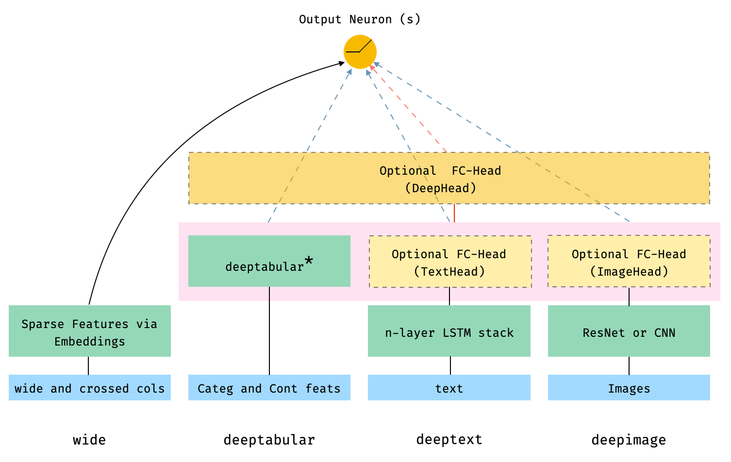
The dashed boxes in the figure represent optional, overall components, and the dashed lines/arrows indicate the corresponding connections, depending on whether or not certain components are present. For example, the dashed, blue-arrows indicate that the deeptabular, deeptext and deepimage components are connected directly to the output neuron or neurons (depending on whether we are performing a binary classification or regression, or a multi-class classification) if the optional deephead is not present. Finally, the components within the faded-pink rectangle are concatenated.
Note that it is not possible to illustrate the number of architectures and components available in pytorch-widedeep in one Figure. This is why I wrote before "overall components", because within the components represented by the boxes, there are a number of options as well. Therefore, for more details on possible architectures (and more) please, see the documentation, or the Examples folders and the notebooks in the repo.
In math terms, and following the notation in the paper, the expression for the architecture without a deephead component can be formulated as:
Where $W$ are the weight matrices applied to the wide model and to the final activations of the deep models, $a$ are these final activations, and $\phi(x)$ are the cross product transformations of the original features $x$. In case you are wondering what are "cross product transformations", here is a quote taken directly from the paper: "For binary features, a cross-product transformation (e.g., “AND(gender=female, language=en)”) is 1 if and only if the constituent features (“gender=female” and “language=en”) are all 1, and 0 otherwise".
While if there is a deephead component, the previous expression turns into:
It is important to emphasize that each individual component, wide, deeptabular, deeptext and deepimage, can be used independently and in isolation. For example, one could use only wide, which is in simply a linear
model. In fact, one of the most interesting offerings in pytorch-widedeep is the deeptabular component, and I intend to write a dedicated post focused on that component alone.
Finally, while I recommend using the wide and deeptabular models in pytorch-widedeep it is very likely that users will want to use their own models for the deeptext and deepimage components. That is perfectly
possible as long as the the custom models have an attribute called output_dim with the size of the last layer of activations, so that WideDeep can be constructed. Again, examples on how to use custom components can be found in the Examples folder in the repo. Just in case pytorch-widedeep includes standard text (stack of LSTMs) and image
(pre-trained ResNets or stack of CNNs) models.
3. Quick start (TL;DR)
Maybe I should have started with this section, but I thought that knowing at least the architectures one can build with pytorch-widedeep was "kind-off" necessary. In any case and before diving into the details of the library, let's just say that you just want to quickly run one example and get the feel of how pytorch-widedeep works. Let's do so using the adult census dataset.
In this example we will be fitting a model comprised by two components: wide and deeptabular.
#collapse-hide
import pandas as pd
import numpy as np
from sklearn.model_selection import train_test_split
from sklearn.metrics import accuracy_score
#collapse-hide
adult = pd.read_csv("data/adult/adult.csv.zip")
adult.columns = [c.replace("-", "_") for c in adult.columns]
adult["income_label"] = (adult["income"].apply(lambda x: ">50K" in x)).astype(int)
adult.drop("income", axis=1, inplace=True)

for c in adult.columns:
    if adult[c].dtype == 'O':
        adult[c] = adult[c].apply(lambda x: "unknown" if x == "?" else x)
        adult[c] = adult[c].str.lower()
adult_train, adult_test = train_test_split(adult, test_size=0.2, stratify=adult.income_label)

adult.head()
The following lines below is all you need
from pytorch_widedeep import Trainer
from pytorch_widedeep.preprocessing import WidePreprocessor, TabPreprocessor
from pytorch_widedeep.models import Wide, TabMlp, WideDeep
from pytorch_widedeep.metrics import Accuracy

# define wide, crossed, embedding and continuous columns, and target
wide_cols = ["education", "relationship", "workclass", "occupation", "native_country", "gender"]
cross_cols = [("education", "occupation"), ("native_country", "occupation")]
embed_cols = [("education", 32), ("workclass", 32), ("occupation", 32), ("native_country", 32)]
cont_cols = ["age", "hours_per_week"]
target = adult_train["income_label"].values

# prepare wide component
wide_preprocessor = WidePreprocessor(wide_cols=wide_cols, crossed_cols=cross_cols)
X_wide = wide_preprocessor.fit_transform(adult_train)
wide = Wide(wide_dim=np.unique(X_wide).shape[0], pred_dim=1)

# prepare deeptabular component
tab_preprocessor = TabPreprocessor(embed_cols=embed_cols, continuous_cols=cont_cols)
X_tab = tab_preprocessor.fit_transform(adult_train)
deeptabular = TabMlp(
    mlp_hidden_dims=[200, 100],
    column_idx=tab_preprocessor.column_idx,
    embed_input=tab_preprocessor.embeddings_input,
    continuous_cols=cont_cols,
)

# build, compile and fit
model = WideDeep(wide=wide, deeptabular=deeptabular)

# Train
trainer = Trainer(model, objective="binary", metrics=[(Accuracy)])
trainer.fit(X_wide=X_wide, X_tab=X_tab, target=target, n_epochs=2, batch_size=256)

# predict
X_wide_te = wide_preprocessor.transform(adult_test)
X_tab_te = tab_preprocessor.transform(adult_test)
preds = trainer.predict(X_wide=X_wide_te, X_tab=X_tab_te)
4. Preprocessors
As you can see in Section 3, and as with any ML algorithm, the data need to be prepared/preprocessed before going through the model. This is handled by the pytorch-widedeep preprocessors. There is one preprocessor per WideDeep model component:
WidePreprocessor
TabPreprocessor
TextPreprocessor
ImagePreprocessor
"Behind the scenes", these preprocessors use a series of helper functions and classes that are in the utils module. Initially I did not intend to "expose" them to the user, but I believe they can be useful for all sorts of preprocessing tasks, even if they are not related to pytorch-widedeep, so I made them available. The utils tools are:
deep_utils.LabelEncoder
text_utils.simple_preprocess
text_utils.get_texts
text_utils.pad_sequences
text_utils.build_embeddings_matrix
fastai_transforms.Tokenizer
fastai_transforms.Vocab
image_utils.SimplePreprocessor
image_utils.AspectAwarePreprocessor
They are accessible directly from utils, e.g.:
from pytorch_widedeep.utils import LabelEncoder
Note that here I will be concentrating directly on the preprocessors. If you want more details on the utils tools, have a look to the source code or read the documentation.
4.1. WidePreprocessor
The Wide component of the model is a linear model that in principle, could be implemented as a linear layer receiving the result of on one-hot encoded categorical columns. However, this is not memory efficient (at all). Therefore, we implement a liner layer as an Embedding layer plus a bias. I will explain it in a bit more detail later. For now, just know that WidePreprocessor simply encodes the categories numerically so that they are the indexes of the lookup table that is an Embedding layer.
from pytorch_widedeep.preprocessing import WidePreprocessor

wide_cols = ['education', 'relationship','workclass','occupation','native_country','gender']
crossed_cols = [('education', 'occupation'), ('native_country', 'occupation')]

wide_preprocessor = WidePreprocessor(wide_cols=wide_cols, crossed_cols=crossed_cols)
X_wide = wide_preprocessor.fit_transform(adult)
# From here on, any new observation can be prepared by simply running `.transform`
# new_X_wide = wide_preprocessor.transform(new_df)
X_wide
X_wide[0]
Note that the label encoding starts from 1. This is because it is convenient to leave 0 for padding, i.e. unknown categories. Let's take from example the first entry
wide_preprocessor.inverse_transform(X_wide[:1])
As we can see, wide_preprocessor numerically encodes the wide_cols and the crossed_cols, which can be recovered using the method inverse_transform.
from pytorch_widedeep.preprocessing import TabPreprocessor

# cat_embed_cols = [(column_name, embed_dim), ...]
cat_embed_cols = [('education',10), ('relationship',8), ('workclass',10), ('occupation',10),('native_country',10)]
continuous_cols = ["age","hours_per_week"]

tab_preprocessor = TabPreprocessor(embed_cols=cat_embed_cols, continuous_cols=continuous_cols)
X_tab = tab_preprocessor.fit_transform(adult)
# From here on, any new observation can be prepared by simply running `.transform`
# new_X_deep = deep_preprocessor.transform(new_df)
print(X_tab[:5])
Note that the label encoding starts from 1. This is because it is convenient to leave 0 for padding, i.e. unknown categories. Let's take from example the first entry
Behind the scenes, TabPreprocessor uses LabelEncoder, simply a custom numerical encoder for categorical features, available via
from pytorch_widedeep.utils import LabelEncoder
4.3. TextPreprocessor
This preprocessor returns the tokenized, padded sequences that will be directly "fed" to the deeptext component.
To illustrate the text and image preprocessors I will use a small sample of the Airbnb listing dataset, which you can get here.
airbnb=pd.read_csv("data/airbnb/airbnb_sample.csv")
texts = airbnb.description.tolist()
texts[0]
from pytorch_widedeep.preprocessing import TextPreprocessor

text_preprocessor = TextPreprocessor(text_col='description')
X_text = text_preprocessor.fit_transform(airbnb)
# From here on, any new observation can be prepared by simply running `.transform`
# new_X_text = text_preprocessor.transform(new_df)
print(X_text[0])
TextPreprocessor uses the utilities within the text_utils and the fastai_transforms modules. Again, all the utilities within those modules are are directly accessible from utils, e.g.:
from pytorch_widedeep.utils import simple_preprocess, pad_sequences, build_embeddings_matrix, Tokenizer, Vocab
4.4 ImagePreprocessor
Finally, ImagePreprocessor simply resizes the images, being aware of the aspect ratio. By default they will be resized to (224, 224, ...). This is because the default deepdense component of the model is a pre-trained ResNet model, which requires inputs of height and width of 224.
Let's have a look
from pytorch_widedeep.preprocessing import ImagePreprocessor

image_preprocessor = ImagePreprocessor(img_col='id', img_path="data/airbnb/property_picture/")
X_images = image_preprocessor.fit_transform(airbnb)
# From here on, any new observation can be prepared by simply running `.transform`
# new_X_images = image_preprocessor.transform(new_df)
X_images[0].shape
ImagePreprocessor uses two helpers: SimplePreprocessor and AspectAwarePreprocessor, available from the utils module, e.g.:
from pytorch_widedeep.utils import SimplePreprocessor, AspectAwarePreprocessor
These two classes are directly taken from Adrian Rosebrock's fantastic book "Deep Learning for Computer Vision". Therefore, all credit to Adrian.
Let's now have a look to the components that can be used to build a wide and deep model. The 5 main components of WideDeep are:
wide
deeptabular
deeptext
deepimage
deephead
The first 4 will be collected and combined by the WideDeep class, while the 5th one can be optionally added to the WideDeep model through its corresponding parameters: deephead or alternatively head_layers, head_dropout and head_batchnorm.
5.1. wide
The wide component is a Linear layer "plugged" into the output neuron(s)
The only particularity of our implementation is that we have implemented the linear layer via an Embedding layer plus a bias. While the implementations are equivalent, the latter is faster and far more memory efficient, since we do not need to one hot encode the categorical features.
Let's have a look:
import torch
import pandas as pd
import numpy as np

from torch import nn
df = pd.DataFrame({'color': ['r', 'b', 'g'], 'size': ['s', 'n', 'l']})
df.head()
one hot encoded, the first observation (color: r, size: s) would be
obs_0_oh = (np.array([1., 0., 0., 1., 0., 0.])).astype('float32')
if we simply numerically encode (or label encode) the values:
obs_0_le = (np.array([0, 3])).astype('int64')
Note that in the implementation of the package we start from 1, saving 0 for padding, i.e. unseen values.
Now, let's see if the two implementations are equivalent
# we have 6 different values. Let's assume we are performing a regression, so pred_dim = 1
lin = nn.Linear(6, 1)
emb = nn.Embedding(6, 1)
emb.weight = nn.Parameter(lin.weight.reshape_as(emb.weight))
lin(torch.tensor(obs_0_oh))
emb(torch.tensor(obs_0_le)).sum() + lin.bias
And this is precisely how the linear component Wide is implemented
from pytorch_widedeep.models import Wide
wide = Wide(wide_dim=10, pred_dim=1)
wide
Again, let me emphasize that even though the input dim is 10, the Embedding layer has 11 weights. This is because we save 0 for padding, which is used for unseen values during the encoding process
5.2. deeptabular
There are 3 alternatives for the so called deepdense component of the model: TabMlp and TabResnet and the TabTransformer:
-
TabMlp: this is almost identical to the tabular model in the fantastic fastai library, and consists simply in embeddings representing the categorical features, concatenated with the continuous features, and passed then through a MLP. -
TabRenset: This is similar to the previous model but the embeddings are passed through a series of ResNet blocks built with dense layers. -
TabTransformer: Details on the TabTransformer can be found in: TabTransformer: Tabular Data Modeling Using Contextual Embeddings
For details on these 3 models and their options please see the examples in the Examples folder and the documentation.
Through the development of the package, the deeptabular component became one of the core values of the package. The possibilities are numerous, and therefore, I will further describe this component in detail in a separate post.
For now let's have a quick look:
Let's have a look first to TabMlp:
from pytorch_widedeep.models import TabMlp

# fake dataset
X_tab = torch.cat((torch.empty(5, 4).random_(4), torch.rand(5, 1)), axis=1)
colnames = ['a', 'b', 'c', 'd', 'e']
embed_input = [(u,i,j) for u,i,j in zip(colnames[:4], [4]*4, [8]*4)]
column_idx = {k:v for v,k in enumerate(colnames)}
continuous_cols = ['e']

# my advice would be to not use dropout in the last layer, but I add the option because you never
# know..there is crazy people everywhere.
tabmlp = TabMlp(
    mlp_hidden_dims=[16,8],
    mlp_dropout=[0.5, 0.],
    mlp_batchnorm=True,
    mlp_activation="leaky_relu",
    column_idx=column_idx,
    embed_input=embed_input,
    continuous_cols=continuous_cols)
tabmlp
tabmlp(X_tab)
Let's now have a look to TabResnet:
from pytorch_widedeep.models import TabResnet

tabresnet = TabResnet(
    blocks_dims=[16, 8],
    blocks_dropout=0.1,
    column_idx=column_idx,
    embed_input=embed_input,
    continuous_cols=continuous_cols,
)


tabresnet
tabresnet(X_tab)
and finally, the TabTransformer:
from pytorch_widedeep.models import TabTransformer
embed_input = [(u,i) for u,i in zip(colnames[:4], [4]*4)]
tabtransformer = TabTransformer(
    column_idx=column_idx,
    embed_input=embed_input,
    continuous_cols=continuous_cols
)
tabtransformer
tabtransformer(X_tab)
5.3. deeptext
pytorch-widedeep offers one model that can be passed to WideDeep as the deeptext component, DeepText, which is a standard and simple stack of LSTMs on top of word embeddings. You could also add a FC-Head on top of the LSTMs. The word embeddings can be pre-trained. In the future I aim to include some simple pre-trained models so that the combination between text and images is fair.
On the other hand, while I recommend using the wide and deeptabular models within this package when building the corresponding wide and deep model components, it is very likely that the user will want to use custom text and image models. That is perfectly possible. Simply, build them and pass them as the corresponding parameters. Note that the custom models MUST return a last layer of activations (i.e. not the final prediction) so that these activations are collected by WideDeep and combined accordingly. In addition, the models MUST also contain an attribute output_dim with the size of these last layers of activations.
I will illustrate all of the above more in detail in the second post of these series.
Let's have a look to DeepText
import torch
from pytorch_widedeep.models import DeepText
X_text = torch.cat((torch.zeros([5,1]), torch.empty(5, 4).random_(1,4)), axis=1)
deeptext = DeepText(vocab_size=4, hidden_dim=4, n_layers=1, padding_idx=0, embed_dim=4)
deeptext
deeptext(X_text)
You could, if you wanted, add a Fully Connected Head (FC-Head) on top of it
deeptext = DeepText(vocab_size=4, hidden_dim=8, n_layers=3, padding_idx=0, embed_dim=4,
                    head_hidden_dims=[8,4], head_batchnorm=True, head_dropout=[0.5, 0.5])
deeptext
deeptext(X_text)
5.4. deepimage
Similarly to deeptext, pytorch-widedeep offers one model that can be passed to WideDeep as the deepimage component, DeepImage, which is either a pre-trained ResNet (18, 34, or 50. Default is 18) or a stack of CNNs, to which one can add a FC-Head. If is a pre-trained ResNet, you can chose how many layers you want to defrost deep into the network with the parameter freeze_n
from pytorch_widedeep.models import DeepImage

X_img = torch.rand((2,3,224,224))
deepimage = DeepImage(head_hidden_dims=[512, 64, 8], head_activation="leaky_relu")

deepimage
deepimage(X_img)
5.5. deephead
The are two possibilities when defining the so-called deephead component.
-
When defining the
WideDeepmodel there is a parameter calledhead_hidden_dims(and the corresponding related parameters. See the package documentation) that define the FC-head on top of thedeeptabular,deeptextanddeepimagecomponents. -
Of course, you could also chose to define it yourself externally and pass it using the parameter
deephead. Have a look at the documentation.
6. Conclusion
This is the first of a series of posts introducing the python library pytorch-widedeep. This library is intended to be a flexible frame to combine tabular data with text and images via wide and deep models. Of course, it can also be used directly on "traditional" tabular data, without text and/or images.
In this post I have shown how to quickly start using the library (Section 3) and explained the utilities available in the preprocessing module (Section 4) and and model component definitions (Section 5), available in the models module.
In the next post I will show more advance uses that hopefully will illustrate pytorch-widedeep's flexibility to build wide and deep models.
References
[1] Wide & Deep Learning for Recommender Systems. Heng-Tze Cheng, Levent Koc, Jeremiah Harmsen, et al. 2016. arXiv:1606.07792
[2] TabNet: Attentive Interpretable Tabular Learning. Sercan O. Arik, Tomas Pfister, 2020. arXiv:1908.07442
[3] AutoGluon-Tabular: Robust and Accurate AutoML for Structured Data Nick Erickson, Jonas Mueller, Alexander Shirkov, et al., 2020. arXiv:2003.06505
[4] Universal Language Model Fine-tuning for Text Classification. Jeremy Howard, Sebastian Ruder, 2018 arXiv:1801.06146v5
[5] Single Headed Attention RNN: Stop Thinking With Your Head. Stephen Merity, 2019 arXiv:1801.06146v5