pytorch-widedeep, deep learning for tabular data II: advanced use
a flexible package to combine tabular data with text and images using wide and deep models.


- 1. Binary classification with varying parameters
- 2. Using the Focal Loss
- 3. Regression combining tabular data, text and images
- 4. Finetune/Warmup routines
- 5. Custom model
- 6. Conclusion
This is the second of a series of posts introducing pytorch-widedeep, a flexible package to combine tabular data with text and images (that could also be used for "standard" tabular data alone).
In the first post I described pytorch-widedeep's data preprocessing utilities, the main components of a WideDeep model and a quick example to illustrate the basic use of the library. In this post I will use a series of examples to dig deeper into the many options pytorch-widedeep offers as we build wide and deep models.
1. Binary classification with varying parameters
Let's start by using again the adult census dataset.
Before moving any further, let me emphasize that, as we go through the examples, one should not pay excessive (or any) attention to the loss or the metrics in the sense that the input parameters are not selected to obtain "state of the art", but to illustrate usability.
A proper benchmarking exercise will be carried out in a future post. Having said that, and without further ado, let's start.
#collapse-hide
import pandas as pd
import numpy as np

adult = pd.read_csv("data/adult/adult.csv.zip")
adult.columns = [c.replace("-", "_") for c in adult.columns]
adult["income_label"] = (adult["income"].apply(lambda x: ">50K" in x)).astype(int)
adult.drop("income", axis=1, inplace=True)

for c in adult.columns:
    if adult[c].dtype == 'O':
        adult[c] = adult[c].apply(lambda x: "unknown" if x == "?" else x)
        adult[c] = adult[c].str.lower()
adult.head()
if you read the first post you will be familiar with the code below:
import torch

from pytorch_widedeep import Trainer
from pytorch_widedeep.preprocessing import WidePreprocessor, TabPreprocessor
from pytorch_widedeep.models import Wide, TabMlp, TabResnet, WideDeep
from pytorch_widedeep.metrics import Accuracy, Recall

wide_cols = ['education', 'relationship','workclass','occupation','native_country','gender']
crossed_cols = [('education', 'occupation'), ('native_country', 'occupation')]
cat_embed_cols = [('education',32), ('relationship',32), ('workclass',32), ('occupation',32),('native_country',32)]
continuous_cols = ["age","hours_per_week"]
target_col = 'income_label'

# TARGET
target = adult[target_col].values

# WIDE
wide_preprocessor = WidePreprocessor(wide_cols=wide_cols, crossed_cols=crossed_cols)
X_wide = wide_preprocessor.fit_transform(adult)

# DEEP
tab_preprocessor = TabPreprocessor(embed_cols=cat_embed_cols, continuous_cols=continuous_cols)
X_tab = tab_preprocessor.fit_transform(adult)
wide = Wide(wide_dim=np.unique(X_wide).shape[0], pred_dim=1)
# We can add dropout and batchnorm to the dense layers, as well as chose the order of the operations
deeptabular = TabMlp(column_idx=tab_preprocessor.column_idx,
                   mlp_hidden_dims=[64,32],
                   mlp_dropout=[0.5, 0.5],
                   mlp_batchnorm=True,
                   mlp_linear_first = True,
                   embed_input=tab_preprocessor.embeddings_input,
                   continuous_cols=continuous_cols)
model = WideDeep(wide=wide, deeptabular=deeptabular)
Let's have a look to the model that we will be running:
model
Now we will define the set up for each model component, including optimizers, learning rate schedulers and initializers:
from pytorch_widedeep.initializers import KaimingNormal, XavierNormal
from pytorch_widedeep.callbacks import ModelCheckpoint, LRHistory, EarlyStopping
from pytorch_widedeep.optim import RAdam
# Optimizers
wide_opt = torch.optim.Adam(model.wide.parameters(), lr=0.03)
deep_opt = RAdam(model.deeptabular.parameters(), lr=0.01)
# LR Schedulers
wide_sch = torch.optim.lr_scheduler.StepLR(wide_opt, step_size=3)
deep_sch = torch.optim.lr_scheduler.StepLR(deep_opt, step_size=5)

# Component-dependent settings as Dict
optimizers = {'wide': wide_opt, 'deeptabular':deep_opt}
schedulers = {'wide': wide_sch, 'deeptabular':deep_sch}
initializers = {'wide': KaimingNormal, 'deeptabular':XavierNormal}

# General settings as List
callbacks = [LRHistory(n_epochs=10), EarlyStopping, ModelCheckpoint(filepath='model_weights/wd_out')]
metrics = [Accuracy, Recall]
Build the trainer and fit!
trainer = Trainer(model,
                  objective='binary',
                  optimizers=optimizers,
                  lr_schedulers=schedulers,
                  initializers=initializers,
                  callbacks=callbacks,
                  metrics=metrics,
                  verbose=0,
                 )
trainer.fit(X_wide=X_wide, X_tab=X_tab, target=target, n_epochs=10, batch_size=256, val_split=0.2)
#collapse-hide
import matplotlib.pyplot as plt
%matplotlib inline

import seaborn as sns
sns.set()
#collapse-hide
plt.figure(figsize=(15,8))
plt.subplot(2,2,1)
plt.plot(trainer.history['train_loss'], label="train")
plt.plot(trainer.history['val_loss'], label="val")
plt.legend(fontsize=13)
plt.xlabel("n epochs", fontsize=13)
plt.ylabel("Loss", fontsize=13)


plt.subplot(2,2,2)
plt.plot(trainer.history['train_acc'], label="train")
plt.plot(trainer.history['val_acc'], label="val")
plt.legend(fontsize=13)
plt.xlabel("n epochs", fontsize=13)
plt.ylabel("Accuracy", fontsize=13)

plt.subplot(2,2,3)
plt.plot(trainer.lr_history['lr_wide_0'], label="wide")
plt.plot(trainer.lr_history['lr_deeptabular_0'], label="deeptabular")
plt.legend(fontsize=13)
plt.xlabel("n epochs", fontsize=13)
plt.ylabel("learning rate", fontsize=13)

As we can see from the plots, the learning rate effectively decreases by a factor of 0.1 (the default) after the corresponding step_size for each component. Note that the keys in the model.lr_history dictionary have a suffix _0. This is because if you pass different parameter groups to the torch optimizers, these will also be recorded. We'll see this in the regression example later in the post.
Before I move to the next section let me just mention that the WideDeep class comes with a useful method to "rescue" the learned embeddings, very creatively called get_embeddings. For example, let's say I want to use the embeddings learned for the different levels of the categorical feature education. These can be access via:
education_embed = trainer.get_embeddings(
    col_name='education',
    cat_encoding_dict=tab_preprocessor.label_encoder.encoding_dict
)
education_embed['doctorate']
2. Using the Focal Loss
The Focal loss (hereafter FL) was introduced by Tsung-Yi Lin et al., in their 2018 paper “Focal Loss for Dense Object Detection” [1]. It is designed to address scenarios with extreme imbalanced classes, such as one-stage object detection where the imbalance between foreground and background classes can be, for example, 1:1000.
The adult census dataset is not really imbalanced, therefore is not the best dataset to test the performance of the FL. Nonetheless, let me illustrate how easy is to use the FL with pytorch-widedeep.
model = WideDeep(wide=wide, deeptabular=deeptabular)
trainer = Trainer(
    model,
    objective="binary_focal_loss",
    optimizers=optimizers,
    lr_schedulers=schedulers,
    initializers=initializers,
    callbacks=callbacks,
    metrics=metrics,
    alpha=0.2, # the alpha parameter of the focal loss
    gamma=1.0, # the gamma parameter of the focal loss
    verbose=False
)
trainer.fit(X_wide=X_wide, X_tab=X_tab, target=target, n_epochs=2, batch_size=256, val_split=0.2)
To learn more about the losses available at pytorch-widedeep have a look at the losses module in the library or the docs.
3. Regression combining tabular data, text and images
For this example we will use a small sample (so you can run it locally in a laptop) of the Airbnb listings dataset in London.
In case you are interested in all details, I did prepared the original dataset for this post, and all the code can be found at the airbnb_data_preprocessing.py, here. After such preprocessing the data looks like this:
#collapse-hide
airbnb = pd.read_csv('data/airbnb/airbnb_sample.csv')
airbnb.head(1)
Let's define what will go through the wide and deep components
# There are a number of columns that are already binary. Therefore, no need to one hot encode them
crossed_cols = [('property_type', 'room_type')]
already_dummies = [c for c in airbnb.columns if 'amenity' in c] + ['has_house_rules']
wide_cols = ['is_location_exact', 'property_type', 'room_type', 'host_gender',
'instant_bookable'] + already_dummies
cat_embed_cols = [(c, 16) for c in airbnb.columns if 'catg' in c] + \
    [('neighbourhood_cleansed', 64), ('cancellation_policy', 16)]
continuous_cols = ['latitude', 'longitude', 'security_deposit', 'extra_people']
# it does not make sense to standarised Latitude and Longitude. Here I am going to "pass" but you
# might want to check the LatLongScalarEnc available in the autogluon tabular library.
already_standard = ['latitude', 'longitude']
# text and image colnames
text_col = 'description'
img_col = 'id'
# path to pretrained word embeddings and the images
word_vectors_path = 'data/glove.6B/glove.6B.100d.txt'
img_path = 'data/airbnb/property_picture'
# target
target_col = 'yield'
Note the following: columns that are already dummies (defined as already_dummies), are treated as any other wide column. Internally, nothing will really happen to them. They will just add one entry to the embedding lookup table.
On the other hand, you will see that among the columns that will be passed through the deeptabular component we have already_standard columns, which are longitude and latitude in this case. These are columns for which it makes no sense to standardize them via sklearn's StandardScaler, which is what TabPreprocessor uses internally. A solution would be to pre-process them before-hand (using for example the LatLongScalarEnc available at the autogluon library) and then pass them to the TabPreprocessor.
Nonetheless, in this case I am going to "ignore" this issue and move on since I just want to illustrate the use of the package.
import os
import torch

from pytorch_widedeep.preprocessing import WidePreprocessor, TabPreprocessor, TextPreprocessor, ImagePreprocessor
from pytorch_widedeep.models import Wide, TabMlp, DeepText, DeepImage, WideDeep
from pytorch_widedeep.initializers import *
from pytorch_widedeep.callbacks import *
target = airbnb[target_col].values

wide_preprocessor = WidePreprocessor(wide_cols=wide_cols, crossed_cols=crossed_cols)
X_wide = wide_preprocessor.fit_transform(airbnb)

tab_preprocessor = TabPreprocessor(embed_cols=cat_embed_cols, continuous_cols=continuous_cols)
X_tab = tab_preprocessor.fit_transform(airbnb)

text_preprocessor = TextPreprocessor(word_vectors_path=word_vectors_path, text_col=text_col)
X_text = text_preprocessor.fit_transform(airbnb)

image_processor = ImagePreprocessor(img_col = img_col, img_path = img_path)
X_images = image_processor.fit_transform(airbnb)
At this stage the data is ready to be passed through the model. However, instead of building a "simple" model that collects the wide, deeptabular, deeptext and deepimage component, I am going to use this opportunity to illustrate pytorch-widedepp's flexibility to build wide and deep models. I like to call this, getting into Kaggle mode.
First we define the components of the model...
wide = Wide(wide_dim=np.unique(X_wide).shape[0], pred_dim=1)

# deeptabular: 2 Dense layers
deeptabular = TabMlp(
    column_idx = tab_preprocessor.column_idx,
    mlp_hidden_dims=[128,64],
    mlp_dropout = 0.1,
    mlp_batchnorm = True,
    embed_input=tab_preprocessor.embeddings_input,
    embed_dropout = 0.1,
    continuous_cols = continuous_cols,
    batchnorm_cont = True
)

# deeptext: a stack of 2 LSTMs
deeptext = DeepText(
    vocab_size=len(text_preprocessor.vocab.itos),
    hidden_dim=64,
    n_layers=2,
    rnn_dropout=0.5,
    embed_matrix=text_preprocessor.embedding_matrix)

# Pretrained Resnet 18 (default is all but last 2 conv blocks frozen) plus a FC-Head 512->256->128
deepimage = DeepImage(pretrained=True, head_hidden_dims=[512, 256, 128])
...and, as we build the model, add a fully connected head via the input parameters (could also be used via the additional component/parameter deephead)
model = WideDeep(
    wide=wide,
    deeptabular=deeptabular,
    deeptext=deeptext,
    deepimage=deepimage,
    head_hidden_dims=[128, 64]
)
Let's have a look to the model
model
This is a big model, so let me go component by component.
-
wide: simple linear model implemented via anEmbeddinglayer -
deeptabular: embeddings concatenated to categorical columns that are then passed through two dense layers with the following sizes [196 $\rightarrow$ 128 $\rightarrow$ 64]. -
deeptext: two stacked LTSMs that will received the pre-trained glove wordvectors and output a last hidden state of dim 64 (this would be 128 if we had usedbidirectional = True) -
deepimage: a pre-trained ResNet 18 model where only the lastSequentialblock (7) will be trained. The rest will remain "frozen". on top of it we haveimageheadwhich is just aSequentialmodel comprised of two dense layers with the following sizes [512 $\rightarrow$ 256 $\rightarrow$ 128] -
deephead: on top of the 3 deep components we have a final component referred asdeephead. This component will receive the concatenated output from all the deep components, and pass it through a further collection of dense layers. In this case the sizes are [256 $\rightarrow$ 64 $\rightarrow$ 1]. We input 256 because the output dim fromdeeptabularis 64, the output dim fromdeeptextis 64 and the output dim fromdeepimageis 128. The finaldeepheadoutput dim is 1 because we are performing a regression, i.e. one output neuron with no activation function.
Let's go even a step further and use different optimizers, initializers and schedulers for different components. Moreover, let's use a different learning rate for different parameter groups in the case of the deeptabular, remember, this is Kaggle mode.
# Optimizers. Different parameter groups for the deeptabular component will use different lr
tab_params = []
for childname, child in model.named_children():
    if childname == 'deeptabular':
        for n,p in child.named_parameters():
            if "emb_layer" in n: tab_params.append({'params': p, 'lr': 0.01})
            else: tab_params.append({'params': p, 'lr': 0.03})

wide_opt = torch.optim.Adam(model.wide.parameters(), lr=0.03)
tab_opt = torch.optim.Adam(tab_params)
text_opt = RAdam(model.deeptext.parameters())
img_opt  = RAdam(model.deepimage.parameters())
head_opt = torch.optim.AdamW(model.deephead.parameters())
optimizers = {'wide': wide_opt, 'deeptabular':tab_opt, 'deeptext':text_opt, 'deepimage': img_opt, 'deephead': head_opt}

# schedulers
wide_sch = torch.optim.lr_scheduler.StepLR(wide_opt, step_size=5)
deep_sch = torch.optim.lr_scheduler.MultiStepLR(tab_opt, milestones=[3,8])
text_sch = torch.optim.lr_scheduler.StepLR(text_opt, step_size=5)
img_sch  = torch.optim.lr_scheduler.MultiStepLR(tab_opt, milestones=[3,8])
head_sch = torch.optim.lr_scheduler.StepLR(head_opt, step_size=5)
schedulers = {'wide': wide_sch, 'deeptabular':deep_sch, 'deeptext':text_sch, 'deepimage': img_sch, 'deephead': head_sch}

# initializers
initializers = {'wide': KaimingNormal, 'deeptabular':KaimingNormal,
                'deeptext':KaimingNormal(pattern=r"^(?!.*word_embed).*$"), # do not initialize the pre-trained word-vectors!
                'deepimage':KaimingNormal}

# transforms and callbacks
mean = [0.406, 0.456, 0.485]  #BGR
std =  [0.225, 0.224, 0.229]  #BGR
transforms = [ToTensor, Normalize(mean=mean, std=std)]
callbacks = [LRHistory(n_epochs=10), EarlyStopping, ModelCheckpoint(filepath='model_weights/wd_out')]
Note that, since we will use pre-trained word embeddings, we do not want to initialize these embeddings. However you might still want to initialize the other layers in the deeptext component. This is not a problem, you can do that with the parameter pattern and your knowledge on regular expressions. In the deeptext initializer definition above:
KaimingNormal(pattern=r"^(?!.*word_embed).*$")
I am NOT initializing parameters whose name contains the string word_embed.
So...let's compile and run, which is as easy as:
trainer = Trainer(model, objective="regression", initializers=initializers, optimizers=optimizers,
    lr_schedulers=schedulers, callbacks=callbacks, transforms=transforms)
trainer.fit(X_wide=X_wide, X_tab=X_tab, X_text=X_text, X_img=X_images,
    target=target, n_epochs=1, batch_size=32, val_split=0.2)
As I mentioned early in the post, please, do not focus on the success metric/loss (mse in this case). I am just using a very small sample of the dataset and some "random" set up. I just want to illustrate usability. A benchmark post will come in the "no-so-distant future".
4. Finetune/Warmup routines
Let's place ourselves in two possible scenarios.
-
Let's assume we have run a model and we want to just transfer the learnings (you know...transfer-learning) to another dataset, or simply we have received new data and we do not want to start the training of each component from scratch. Simply, we want to load the pre-trained weights and fine-tune.
-
Or, we just want to "warm up" individual model components individually before the joined training begins.
This can be done with the finetune set of parameters (aliased all as warmup parameters if you wanted). There are 3 fine-tuning routines:
-
Fine-tune all trainable layers at once with a triangular one-cycle learning rate (referred as slanted triangular learning rates in Howard & Ruder 2018)
-
Gradual fine-tuning inspired by the work of Felbo et al., 2017 [2]
-
Gradual fine-tuning based on the work of Howard & Ruder 2018 [3]
Currently fine-tunning is only supported without a fully connected head, i.e. if deephead=None. In addition, Felbo and Howard routines apply only, of course, to the deeptabular, deeptext and deepimagemodels. The wide component can also be fine-tuned, but only in an "all at once" mode.
Let me briefly describe the "Felbo" and "Howard" routines before showing how to use them.
4.1 The Felbo finetune routine
The Felbo fine-tune routine can be illustrated by the following figure:
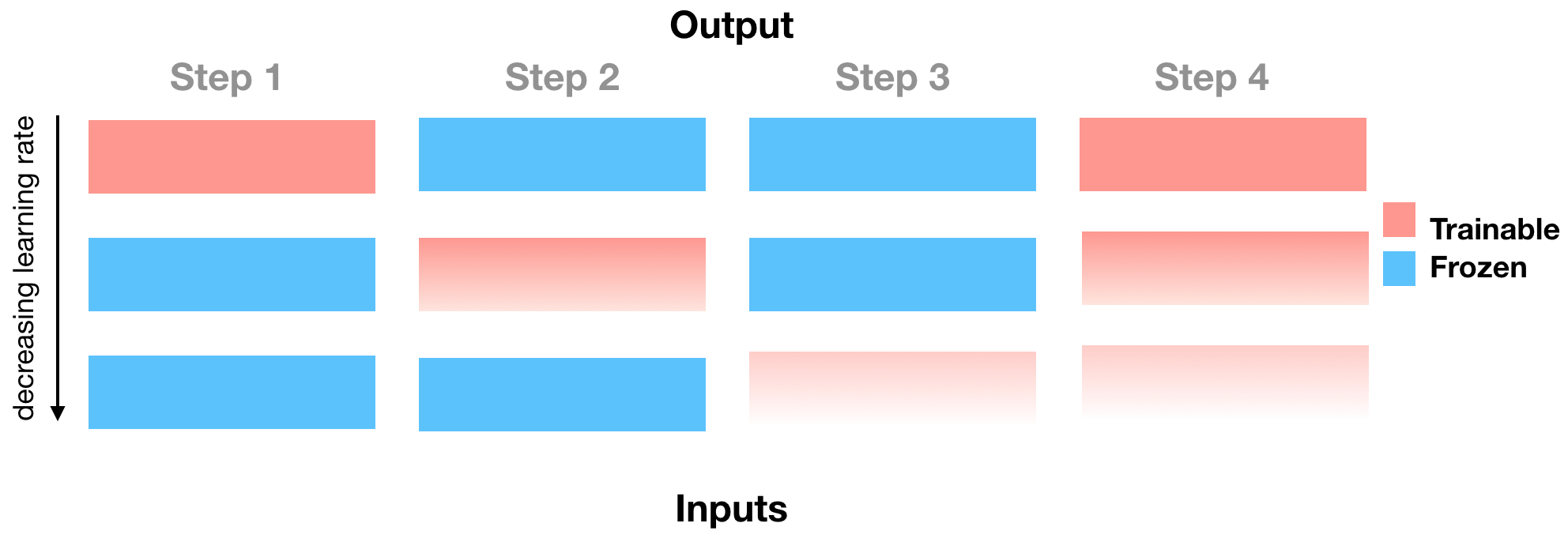
Figure 1. The figure can be described as follows: fine-tune (or train) the last layer for one epoch using a one cycle triangular learning rate. Then fine-tune the next deeper layer for one epoch, with a learning rate that is a factor of 2.5 lower than the previous learning rate (the 2.5 factor is fixed) while freezing the already warmed up layer(s). Repeat untill all individual layers are warmed. Then warm one last epoch with all warmed layers trainable. The vanishing color gradient in the figure attempts to illustrate the decreasing learning rate.
Note that this is not identical to the Fine-Tunning routine described in Felbo et al, 2017, this is why I used the word 'inspired'.
4.2 The Howard finetune routine
The Howard routine can be illustrated by the following figure:
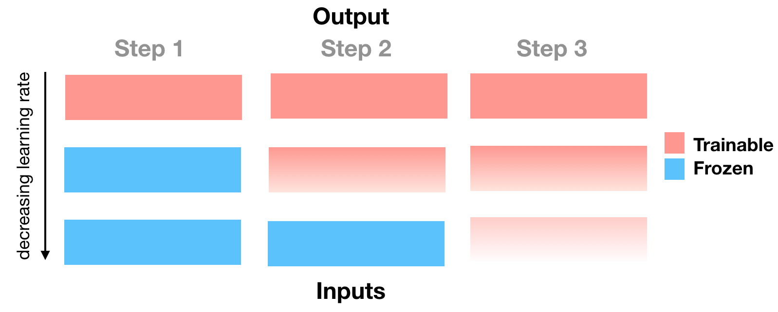
Figure 2. The figure can be described as follows: fine-tune (or train) the last layer for one epoch using a one cycle triangular learning rate. Then fine-tune the next deeper layer for one epoch, with a learning rate that is a factor of 2.5 lower than the previous learning rate (the 2.5 factor is fixed) while keeping the already warmed up layer(s) trainable. Repeat. The vanishing color gradient in the figure attempts to illustrate the decreasing learning rate.
Note that I write "fine-tune (or train) the last layer for one epoch [...]". However, in practice the user will have to specify the order of the layers to be fine-tuned. This is another reason why I wrote that the fine-tune routines I have implemented are inspired by the work of Felbo and Howard and not identical to their implemenations.
The felbo and howard routines can be accessed with via the finetune parameters (aliased as warmup parameters in case the user wants to use consistent naming). Let me go back to the adult dataset and let's have a look:
wide_cols = ['education', 'relationship','workclass','occupation','native_country','gender']
crossed_cols = [('education', 'occupation'), ('native_country', 'occupation')]
cat_embed_cols = [('education',32), ('relationship',32), ('workclass',32), ('occupation',32),('native_country',32)]
continuous_cols = ["age","hours_per_week"]
target_col = 'income_label'

# TARGET
target = adult[target_col].values

# WIDE
wide_preprocessor = WidePreprocessor(wide_cols=wide_cols, crossed_cols=crossed_cols)
X_wide = wide_preprocessor.fit_transform(adult)

# DEEP
tab_preprocessor = TabPreprocessor(embed_cols=cat_embed_cols, continuous_cols=continuous_cols)
X_tab = tab_preprocessor.fit_transform(adult)
wide = Wide(wide_dim=np.unique(X_wide).shape[0], pred_dim=1)
deeptabular = TabResnet(
    blocks_dims=[128, 64, 32],
    column_idx=tab_preprocessor.column_idx,
    embed_input=tab_preprocessor.embeddings_input,
    continuous_cols=continuous_cols)
model = WideDeep(wide=wide, deeptabular=deeptabular)
model
trainer = Trainer(model, objective="binary", metrics=[Accuracy])
trainer.fit(X_wide=X_wide, X_tab=X_tab, target=target, val_split=0.1, n_epochs=2, batch_size=256)
trainer.save_model("models_dir/model.t")
Now we are going to fine-tune the model components, and in the case of the deeptabular component, we will fine-tune the resnet-blocks and the linear layer but NOT the embeddings.
For this, we need to access the model component's children: deeptabular $\rightarrow$ tab_resnet $\rightarrow$ dense_resnet $\rightarrow$ blocks
# you can just load the model as any pytorch model or use the Trainer's staticmethod `load_model`
model = Trainer.load_model("models_dir/model.t")
tab_lin_layers = list(model.deeptabular.children())[1]
tab_deep_layers = list(
    list(list(list(model.deeptabular.children())[0].children())[2].children())[
        0
    ].children()
)[::-1][:2]
tab_layers = [tab_lin_layers] + tab_deep_layers
tab_layers
new_trainer = Trainer(model, objective="binary", metrics=[Accuracy])
new_trainer.fit(
    X_wide=X_wide,
    X_tab=X_tab,
    target=target,
    val_split=0.1,
    finetune=True,
    finetune_epochs=2,
    finetune_deeptabular_gradual=True,
    finetune_deeptabular_layers = tab_layers,
    finetune_deeptabular_max_lr = 0.01,
    n_epochs=2)
5. Custom model
So far we have used the components that come with pytorch-widedee. However, as I mentioned in the first post, it is very likely that the user wants to use custom models for the deeptext and deepimage components. This is easily attainable by...well...simply passing your own model.
You should just remember that the model must return the last layer of activations (and NOT the predictions) and must contained an attribute called output_dim with the output dimension of that last layer.
For example, let's say we want to use as deeptext a very simple stack of 2 bidirectional GRUs. Let's see how to do such a thing with the airbnb dataset
crossed_cols = [('property_type', 'room_type')]

already_dummies = [c for c in airbnb.columns if 'amenity' in c] + ['has_house_rules']

wide_cols = ['is_location_exact', 'property_type', 'room_type', 'host_gender',
'instant_bookable'] + already_dummies

cat_embed_cols = [(c, 16) for c in airbnb.columns if 'catg' in c] + \
    [('neighbourhood_cleansed', 64), ('cancellation_policy', 16)]

continuous_cols = ['latitude', 'longitude', 'security_deposit', 'extra_people']

already_standard = ['latitude', 'longitude']

text_col = 'description'

img_col = 'id'
word_vectors_path = 'data/glove.6B/glove.6B.100d.txt'

img_path = 'data/airbnb/property_picture'

target_col = 'yield'

target = airbnb[target_col].values

wide_preprocessor = WidePreprocessor(wide_cols=wide_cols, crossed_cols=crossed_cols)
X_wide = wide_preprocessor.fit_transform(airbnb)

tab_preprocessor = TabPreprocessor(embed_cols=cat_embed_cols, continuous_cols=continuous_cols)
X_tab = tab_preprocessor.fit_transform(airbnb)

text_preprocessor = TextPreprocessor(word_vectors_path=word_vectors_path, text_col=text_col)
X_text = text_preprocessor.fit_transform(airbnb)

image_processor = ImagePreprocessor(img_col = img_col, img_path = img_path)
X_images = image_processor.fit_transform(airbnb)
from torch import nn


class MyDeepText(nn.Module):
    def __init__(self, vocab_size, padding_idx=1, embed_dim=100, hidden_dim=64):
        super(MyDeepText, self).__init__()

        # word/token embeddings
        self.word_embed = nn.Embedding(
            vocab_size, embed_dim, padding_idx=padding_idx
        )

        # stack of RNNs
        self.rnn = nn.GRU(
            embed_dim,
            hidden_dim,
            num_layers=2,
            bidirectional=True,
            batch_first=True,
        )

        # Remember, this must be defined. If not WideDeep will through an error
        self.output_dim = hidden_dim * 2

    def forward(self, X):
        embed = self.word_embed(X.long())
        o, h = self.rnn(embed)
        return torch.cat((h[-2], h[-1]), dim=1)
And from here, "proceed as usual"
wide = Wide(wide_dim=np.unique(X_wide).shape[0], pred_dim=1)
deeptabular = TabMlp(
    mlp_hidden_dims=[64,32],
    column_idx=tab_preprocessor.column_idx,
    embed_input=tab_preprocessor.embeddings_input,
    continuous_cols=continuous_cols
)
mydeeptext = MyDeepText(vocab_size=len(text_preprocessor.vocab.itos))
model = WideDeep(wide=wide, deeptabular=deeptabular, deeptext=mydeeptext)
model
trainer = Trainer(model, objective="regression")
trainer.fit(X_wide=X_wide, X_tab=X_tab, X_text=X_text, target=target, n_epochs=1, batch_size=64, val_split=0.2)
6. Conclusion
In this second post I tried to illustrate in detail the different functionalities of the pytorch-widedeep package, and how these can be used to customize each of the four potential components of the WideDeep model that can be built with pytorch-widedeep. I have also describe the warm-up routines that can be used to "warm-up" each individual component before the joined training and finally, how custom models, "external" to pytorch-widedeep can be used in combination with the package.
However, this is not the end of the journey. As you will have seen, there is an "imbalance in the pytorch-widedeep force", in the sense that while fully pre-trained models are incorporated for the deepimage component, this is not the case for the deeptext component, where only pre-trained word embeddings are considered. Of course, as illustrated in Section 4, you could build your own pre-trained deeptext component and pass it to the WideDeep constructor class, but eventually, I want to allow that option within the package.
This means that eventually I will need to integrate the library with some of the pre-trained Language models available or simply code a custom version for pytorch-widedeep.
One the other hand, I want to bring more DL models for the deeptabular components, such as TabNet. There is already a fantastic Pytorch implementation which I highly recommend.
If you made it this far, thanks for reading! And if you use the package, let me know your thoughts!
References
[1] Tsung-Yi Lin, Priya Goyal, Ross Girshick, et al., 2018: Focal Loss for Dense Object Detection. arXiv:1708.02002v2
[3] Using millions of emoji occurrences to learn any-domain representations for detecting sentiment, emotion and sarcasm. Bjarke Felbo, Alan Mislove, Anders Søgaard, et al., 2017. arXiv:1708.00524
[3] Universal Language Model Fine-tuning for Text Classification. Jeremy Howard, Sebastian Ruder, 2018 arXiv:1801.06146v5