pytorch-widedeep, deep learning for tabular data III: the deeptabular component
a flexible package to combine tabular data with text and images using wide and deep models.


This is the third of a series of posts introducing pytorch-widedeep, a flexible package to combine tabular data with text and images (that could also be used for "standard" tabular data alone).
While writing this post I will assume that the reader is not familiar with the previous two posts. Of course, reading them would help, but in order to understand the content of this post and then being able to use pytorch-widedeep on tabular data, is not a requirement.
To start with, as always, just install the package:
pip install pytorch-widedeep
This will install v0.4.8, hopefully the last beta version*. Code-wise I think this could be already v1, but before that I want to try it in a few more datasets and select good default values. In addition, I also intend to implement other algorithms, in particular TabNet [1], for which a very nice implementation already exists.
Moving on, and as I mentioned earlier, pytorch-widedeep's main goal is to facilitate the combination of images and text with tabular data via wide and deep models. To that aim, wide and deep models can be built with up to four model components: wide, deeptabular, deeptext and deepimage, that will take care of the different types of input datasets ("standard" tabular, i.e. numerical and categorical features, text and images). This post focuses only on the so-called deeptabular component, and the 3 different models available in this library that can be used to build that component. Nonetheless, and for completion, I will briefly describe the remaining components first.
The wide component of a wide and deep model is simply a liner model, and in pytorch-widedeep such model can be created via the Wide class. In the case of the deeptext component, pytorch-widedeep offers one model, available via the DeepText class. DeepText builds a simple stack of LSTMs, i.e. a standard DL text classifier or regressor, with flexibility regarding the use of pre-trained word embeddings, of a Fully Connected Head (FC-Head), etc. For the deepimage component, pytorch-widedeep includes two alternatives: a pre-trained Resnet model or a "standard" stack of CNNs to be trained from scratch. The two are available via the DeepImage class which, as in the case of DeepText, offers some flexibility when building the architecture.
To clarify the use of the term "model" and Wide and Deep "model component" (in case there is some confusion), let's have a look to the following code:
wide_model = Wide(...)
text_model = DeepText(...)
image_model = DeepImage(...)

# we use the previous models as the wide and deep model components
wdmodel = WideDeep(wide=wide_model, deeptext=text_model, deepimage=image_model)

...
Simply, a wide and deep model has model components that are (of course) models themselves. Note that any of the four wide and deep model components can be a custom model by the user. In fact, while I recommend using the models available in pytorch-widedeep for the wide and deeptabular model components, it is very likely that users will want to use their own models for the deeptext and deepimagecomponents. That is perfectly possible as long as the custom models have an attribute called output_dim with the size of the last layer of activations, so that WideDeep can be constructed (see this example notebook in the repo). In addition, any of the four components can be used independently in isolation. For example, you might want to use just a wide component, which is simply a linear model. To that aim, simply:
wide_model = Wide(...)

# this would not be a wide and deep model but just wide
wdmodel = WideDeep(wide=wide_model)

...
If you want to learn more about different model components and the models available in pytorch-widedeep please, have a look to the Examples folder in the repo, the documentation or the companion posts. Let's now take a deep dive into the models available for the deeptabular component
$^*$ check the repo or this post for a caveat in the installation if you are using Mac, python 3.8 or Pytorch 1.7+. Note that this is not directly related with the package, but the interplay between Mac and OpenMP, and the new defaults of the multiprocessing library for Mac).
1. The deeptabular component
As I was developing the package I realised that perhaps one of the most interesting offerings in pytorch-widedeep was related to the models available for the deeptabular component. Remember that each component can be used independently in isolation. Building a WideDeep model comprised only by a deeptabular component would be what is normally referred as DL for tabular data. Of course, such model is not a wide and deep model, is "just" deep.
Currently, pytorch-widedeep offers three models that can be used as the deeptabular component. In order of complexity, these are:
-
TabMlp: this is very similar to the tabular model in the fantastic fastai library, and consists simply in embeddings representing the categorical features, concatenated with the continuous features, and passed then through a MLP. -
TabRenset: This is similar to the previous model but the embeddings are passed through a series of ResNet blocks built with dense layers. -
TabTransformer: Details on the TabTransformer can be found in: TabTransformer: Tabular Data Modeling Using Contextual Embeddings. Again, this is similar to the models before but the embeddings are passed through a series of Transformer encoder blocks.
A lot has been (and is being) written about the use of DL for tabular data, and certainly each of these models would deserve a post themselves. Here, I will try to describe them with some detail and illustrate their use within pytorch-widedeep. A proper benchmark exercise will be carried out in a not-so-distant future.
1.1 TabMlp
The following figure illustrates the TabMlp model architecture.
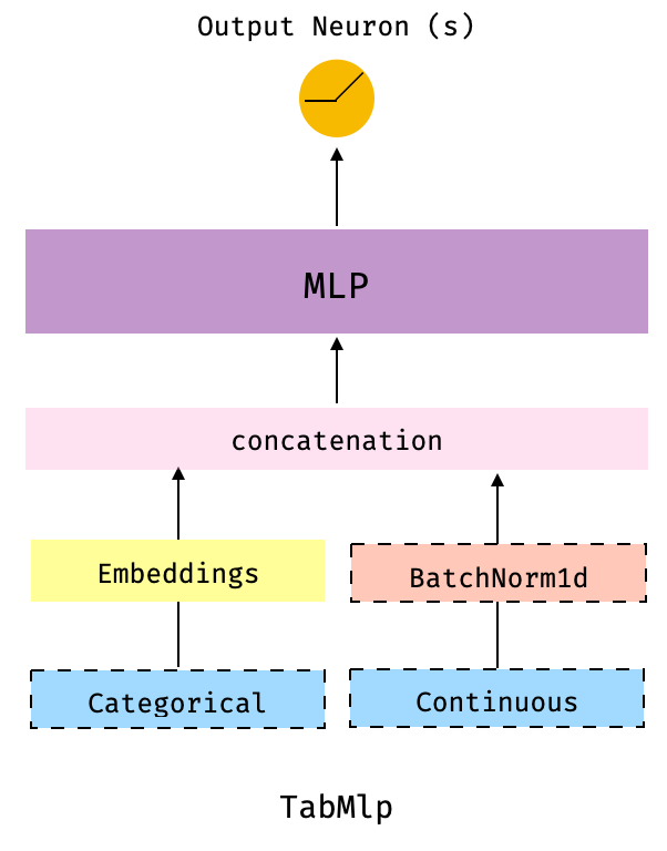
Fig 1. The TabMlp: this is the simples architecture and is very similar to the tabular model available in the fantastic fastai library. In fact, the implementation of the dense layers of the MLP is mostly identical to that in that library.
The dashed-border boxes indicate that these components are optional. For example, we could use TabMlp without categorical components, or without continuous components, if we wanted.
Let's have a look and see how this model is used with the well known adult census dataset. I assume you have downloaded the data and place it at data/adult/adult.csv.zip:
#collapse-hide
import pandas as pd
import numpy as np
from sklearn.model_selection import train_test_split

adult = pd.read_csv("data/adult/adult.csv.zip")
adult.columns = [c.replace("-", "_") for c in adult.columns]
adult["income_label"] = (adult["income"].apply(lambda x: ">50K" in x)).astype(int)
adult.drop("income", axis=1, inplace=True)

for c in adult.columns:
    if adult[c].dtype == 'O':
        adult[c] = adult[c].apply(lambda x: "unknown" if x == "?" else x)
        adult[c] = adult[c].str.lower()
adult_train, adult_test = train_test_split(adult, test_size=0.2, stratify=adult.income_label)
adult.head()
# define the embedding and continuous columns, and target
embed_cols = [
    ('workclass', 6),
    ('education', 8),
    ('marital_status', 6),
    ('occupation',8),
    ('relationship', 6),
    ('race', 6)]
cont_cols = ["age", "hours_per_week", "fnlwgt", "educational_num"]
target = adult_train["income_label"].values
# prepare deeptabular component
from pytorch_widedeep.preprocessing import TabPreprocessor
tab_preprocessor = TabPreprocessor(embed_cols=embed_cols, continuous_cols=cont_cols)

X_tab = tab_preprocessor.fit_transform(adult_train)
Let's pause for a second, since the code up until here is going to be common to all models with some minor adaptations for the TabTransformer. So far, we have simply defined the columns that will be represented by embeddings and the numerical (aka continuous) columns. Once they are defined the dataset is prepared with the TabPreprocessor. Internally, the preprocessor label encodes the "embedding columns" and standardizes the numerical columns. Note that one could chose not to standardizes the numerical columns and then use a BatchNorm1D layer when building the model. That is also a valid approach. Alternatively, one could use both, as I will.
At this stage the data is prepared and we are ready to build the model
from pytorch_widedeep.models import TabMlp, WideDeep

tabmlp = TabMlp(
    mlp_hidden_dims=[200, 100],
    column_idx=tab_preprocessor.column_idx,
    embed_input=tab_preprocessor.embeddings_input,
    continuous_cols=cont_cols,
    batchnorm_cont=True,
)
Let's have a look to the model we just built and how it relates to Fig 1
tabmlp
As we can see, we have a series of columns that would be represented as embeddings. The embeddings from all these columns are concatenated, to form a tensor of dim (bsz, 40) where bsz is batch size. Then, the "batchnormed" continuous columns are also concatenated, resulting in a tensor of dim (bsz, 44), that will be passed to the 2-layer MLP (200 -> 100). In summary Embeddings + continuous+ MLP.
One important thing to mention, common to all models, is that pytorch-widedeep models do not build the last connection, i.e. the connection with the output neuron or neurons depending whether this is a regression, binary or multi-class classification. Such connection is built by the WideDeep constructor class. This means that even if we wanted to use a single-component model, the model still needs to be built with the WideDeep class.
This is because the library is, a priori, intended to build WideDeep models (and hence its name). Once the model is built it is passed to the Trainer (as we will see now). The Trainer class is coded to receive a parent model of class WideDeep with children that are the model components. This is very convenient for a number of aspects in the library.
Effectively this simply requires one extra line of code.
model = WideDeep(deeptabular=tabmlp)
model
As we can see, our model has the final connection now and is a model of class WideDeep formed by one single component, deeptabular, which is a model of class TabMlp formed mainly by the embed_layers and an MLP very creatively called tab_mlp.
We are now ready to train it. The code below simply runs with defaults. one could use any torch optimizer, learning rate schedulers, etc. Just have a look to the docs or the Examples folder in the repo.
from pytorch_widedeep import Trainer
from pytorch_widedeep.metrics import Accuracy

trainer = Trainer(model, objective="binary", metrics=[(Accuracy)])
trainer.fit(X_tab=X_tab, target=target, n_epochs=5, batch_size=256, val_split=0.2)
Once we understand what TabMlp does, TabResnet should be pretty straightforward
1.2 TabResnet
The following figure illustrates the TabResnet model architecture.
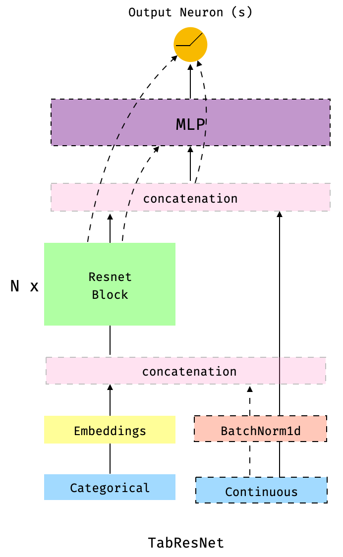
Fig 2. The TabResnet: this model is similar to the TabMlp, but the embeddings (or the concatenation of embeddings and continuous features, normalised or not) are passed through a series of Resnet blocks built with dense layers. The dashed-border boxes indicate that the component is optional and the dashed lines indicate the different paths or connections present depending on which components we decide to include.
This is probably the most flexible of the three models discussed in this post in the sense that there are many variants one can define via the parameters. For example, we could chose to concatenate the continuous features, normalized or not via a BatchNorm1d layer, with the embeddings and then pass the result of such a concatenation trough the series of Resnet blocks. Alternatively, we might prefer to concatenate the continuous features with the results of passing the embeddings through the Resnet blocks. Another optional component is the MLP before the output neuron(s). If not MLP is present, the output from the Resnet blocks or the results of concatenating that output with the continuous features (normalised or not) will be connected directly to the output neuron(s).
Each of the Resnet block is comprised by the following operations:
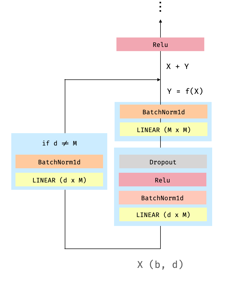
Fig 3. "Dense" Resnet Block. b is the batch size and d the dimension of the embeddings.
Let's build a TabResnet model:
from pytorch_widedeep.models import TabResnet

tabresnet = TabResnet(
    column_idx=tab_preprocessor.column_idx,
    embed_input=tab_preprocessor.embeddings_input,
    continuous_cols=cont_cols,
    batchnorm_cont=True,
    blocks_dims=[200, 100, 100],
    mlp_hidden_dims=[100, 50],
)
model = WideDeep(deeptabular=tabresnet)
model
As we did previously with the TabMlp, let's "walk through" the model. In this case, model is an instance of a WideDeep object formed by a single component, deeptabular that is a TabResnetmodel. TabResnet is formed by a series of Embedding layers (e.g. emb_layer_education) a series of so-called dense Resnet blocks (tab_resnet) and a MLP (tab_resnet_mlp). The embeddings are concatenated themselves and then, further concatenated with the normalised continuous columns. The resulting tensor of dim (bsz, 44) is then passed through two dense Resnet blocks. The output of one Resnet block is the input of the next. Therefore, when setting blocks_dim = [200, 100, 100] we are generating two blocks with input/output 200/100 and 100/100 respectively. The output of the second Resnet blocks, of dim (bsz, 100) is passed through tab_resnet_mlp , the 2-layer MLP, and finally "plugged" into the output neuron. In summary: Embeddings + continuous + dense Renset + MLP.
To run it, the code is, as one might expect identical to the one shown before for the TabMlp.
trainer = Trainer(model, objective="binary", metrics=[(Accuracy)])
trainer.fit(X_tab=X_tab, target=target, n_epochs=5, batch_size=256, val_split=0.2)
And now, last but not least, the last addition to the library, the TabTransformer.
1.3 TabTransformer
The TabTransformer is described in detail in TabTransformer: Tabular Data Modeling Using Contextual Embeddings [2], by the clever guys at Amazon. Is an entertaining paper that I, of course, strongly recommend if you are going to use this model on your tabular data (and also in general if you are interested in DL for tabular data).
My implementation is not the only one available. Given that the model was conceived by the researchers at Amazon, it is also available in their fantastic autogluon library (which you should definitely check). In addition, you can find another implementation here by Phil Wang, whose entire github is simply outstanding. My implementation is partially inspired by these but has some particularities and adaptations so that it works within the pytorch-widedeep package.
The following figure illustrates the TabTransformer model architecture.
![]()
Fig 4. The TabTransfomer, described in TabTransformer: Tabular Data Modeling Using Contextual Embeddings. The dashed-border boxes indicate that the component is optional.
As in previous cases, there are a number of variants and details to consider as one builds the model. I will describe some here, but for a full view of all the possible parameters, please, have a look to the docs.
I don't want to go into the details of what is a Transformer [3] in this post. There is an overwhelming amount of literature if you wanted to learn about it, with the most popular being perhaps The Annotated Transformer. Also check this post and if you are a math "maniac" you might like this paper [4]. However, let me just briefly describe it here so I can introduce the little math we will need for this post. In one sentence, a Transformer consists of a multi-head self-attention layer followed by feed-forward layer, with element-wise addition and layer-normalization being done after each layer.
As most of you will know, a self-attention layer comprises three matrices, Key, Query and Value. Each input categorical column, i.e. embedding, is projected onto these matrices (although see the fixed_attention option later in the post) to generate their corresponding key, query and value vectors. Formally, let $K \in R^{e \times d}$, $Q \in R^{e \times d}$ and $V \in R^{e \times d}$ be the Key, Query and Value matrices of the embeddings where $e$ is the embeddings dimension and $d$ is the dimension of all the Key, Query and Value matrices. Then every input categorical column, i.e embedding, attends to all other categorical columns through an attention head:
where
$$ A = softmax( \frac{QK^T}{\sqrt{d}} ), \hspace{6cm}(2) $$And that is all the math we need.
As I was thinking in a figure to illustrate a transformer block, I realised that there is a chance that the reader has seen every possible representation/figure. Therefore, I decided to illustrate the transformer block in a way that relates directly to the way it is implemented.
![]()
Fig 5. The Transfomer block. The letters in parenthesis indicate the dimension of the corresponding tensor after the operation indicated in the corresponding box. For example, the tensor attn_weights has dim (b, h, s, s).
As the figure shows, the input tensor ($X$) is projected onto its key, query and value matrices. These are then "re-arranged into" the multi-head self-attention layer where each head will attend to part of the embeddings. We then compute $A$ (Eq 2), which is then multiplied by $V$ to obtain what I refer as attn_score (Eq 1). attn_score is then re-arranged, so that we "collect" the attention scores from all the heads, and projected again to obtain the results (attn_out), that will be added to the input and normalised (Y). Finally Y goes through the Feed-Forward layer and a further Add + Norm.
Before moving to the code related to building the model itself, there are a couple of details in the implementation that are worth mentioning
FullEmbeddingDropout
when building a TabTransformer model, there is the possibility of dropping entirely the embedding corresponding to a categorical column. This is set by the parameter full_embed_dropout: bool, which points to the class FullEmbeddingDropout.
SharedEmbeddings
when building a TabTransformer model, it is possible for all the embeddings that represent a categorical column to share a fraction of their embeddings, or define a common separated embedding per column that will be added to the column's embeddings.
The idea behind this so-called "column embedding" is to enable the model to distinguish the classes in one column from those in the other columns. In other words, we want the model to learn representations not only of the different categorical values in the column, but also of the column itself. This is attained by the shared_embed group of parameters: share_embed : bool, add_shared_embed: bool and frac_shared_embed: int. The first simply indicates if embeddings will be shared, the second sets the sharing strategy and the third one the fraction of the embeddings that will be shared, depending on the strategy. They all relate to the class SharedEmbeddings
For example, let's say that we have a categorical column with 5 different categories that will be encoded as embeddings of dim 8. This will result in a lookup table for that column of dim (5, 8). The two sharing strategies are illustrated in Fig 6.
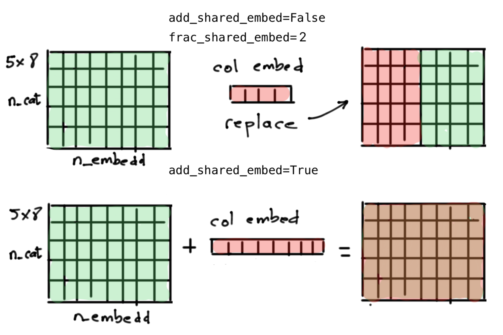 Fig 6. The two sharing embeddings strategies. Upper panel: the "column embedding" replaces
 embedding dim / frac_shared_embed (4 in this case) of the total embeddings that represent the different values of the categorical column. Lower panel: the "column embedding" is added (well, technically broadcasted and added) to the original embedding lookup table. Note that n_cat here refers to the number of different categories for this particular column.
fixed_attention
fixed_attention: this in inspired by the implementation at the Autogluon library. When using "fixed attention", the key and query matrices are not the result of any projection of the input tensor $X$, but learnable matrices (referred as fixed_key and fixed_query) of dim (number of categorical columns x embeddings dim) defined separately, as you instantiate the model. fixed_attention does not affect how the Value matrix is computed.
Let me go through an example with numbers to clarify things. Let's assume we have a dataset with 5 categorical columns that will be encoded by embeddings of dim 4 and we use a batch size (bsz) of 6. Figure 7 shows how the key matrix will be computed for a given batch (same applies to the query matrix) with and without fixed attention.
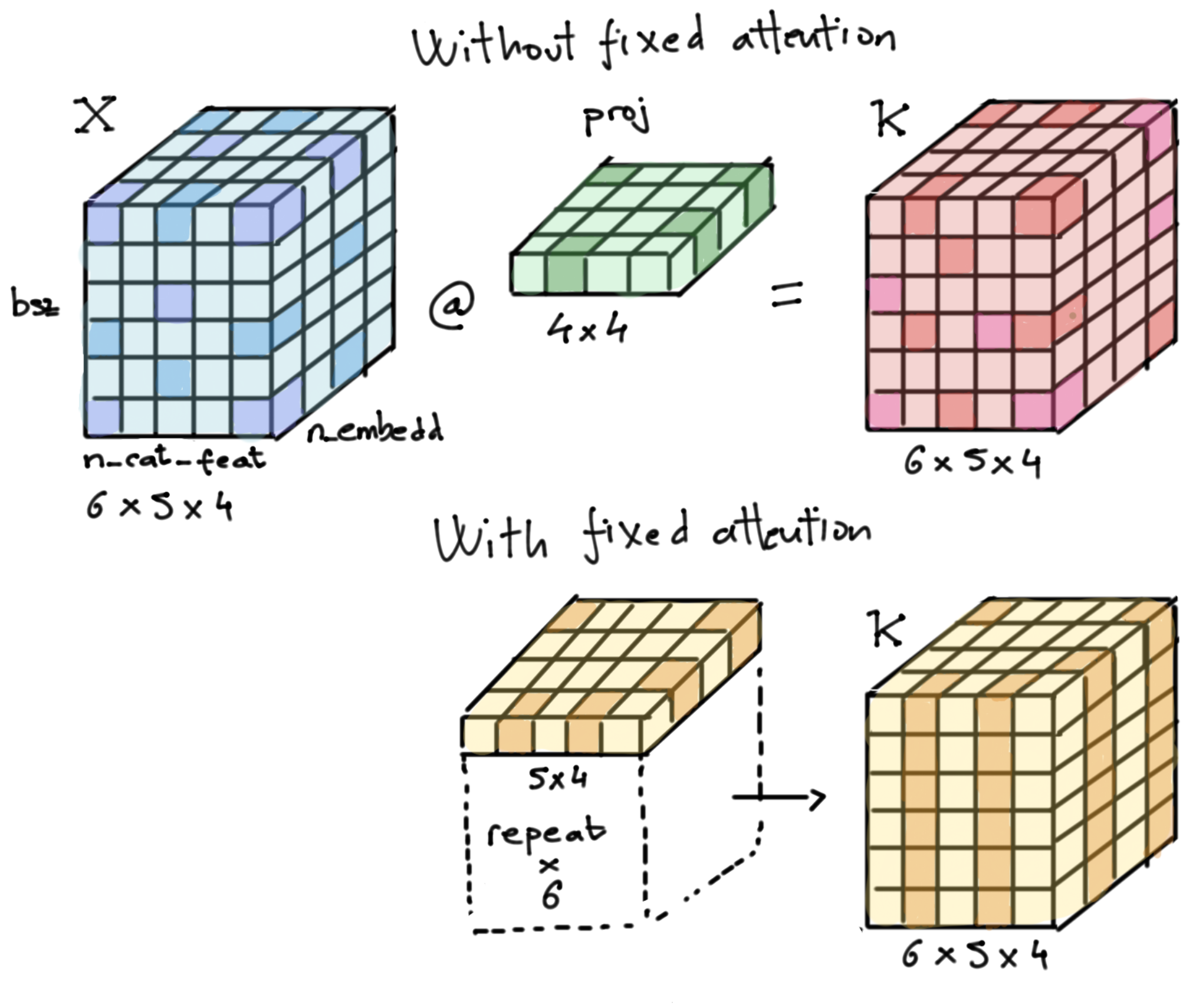 Fig 7. Key matrix computation for a given batch with and without fixed attention (same applies to the query matrix). The different color tones in the matrices are my attempt to illustrate that, while without fixed attention the key matrix can have different values anywhere in the matrix, with fixed attention the key matrix is the result of the repetition of the "fixed-key"
 bsz times. The project-layer is, of course, broadcasted along the bsz dimension in the upper panel.
As I mentioned, this implementation is inspired by that at the Autogluon library. Since the guys at Amazon are the ones that came up with the TabTransformer, is only logical to think that they found a use for this implementation of attention. However, at the time of writing such use is not 100% clear to me. It is known that, in problems like machine translation, most attention heads learn redundant patterns (see e.g. Alessandro Raganato et al., 2020 [5] and references therein). Therefore, maybe the fixed attention mechanism discussed here helps reducing redundancy for problems involving tabular data.
Overall, the way I interpret fixed_attention in layman's terms, is the following: when using fixed attention, the Key and the Query matrices are defined as the model is instantiated, and do not know of the input until the attention weights (attn_weights) are multiplied by the value matrix to obtain what I refer as attn_score in figure 5. Those attention weights, which are in essence the result of a matrix multiplication between the key and the query matrices (plus softmax and normalization), are going to be the same for all the heads, for all samples in a given batch. Therefore, my interpretation is that when using fixed attention, we reduce the attention capabilities of the transformer, which will focus on less aspects of the inputs, reducing potential redundancies.
Anyway, enough speculation. Time to have a look to the code. Note that, since we are going to stack the embeddings (instead of concatenating them) they all must have the same dimensions. Such dimension is set as we build the model instead that at the pre-processing stage. To avoid input format conflicts we use the for_tabtransformer parameter at pre-processing time.
embed_cols = ['workclass', 'education', 'marital_status', 'occupation', 'relationship', 'race']
tab_preprocessor = TabPreprocessor(
    embed_cols=embed_cols,
    continuous_cols=cont_cols,
    for_tabtransformer=True)

X_tab = tab_preprocessor.fit_transform(adult_train)
from pytorch_widedeep.models import TabTransformer

tabtransformer = TabTransformer(
    column_idx=tab_preprocessor.column_idx,
    embed_input=tab_preprocessor.embeddings_input,
    continuous_cols=cont_cols,
    shared_embed=True,
    num_blocks=3,
)
model = WideDeep(deeptabular=tabtransformer)
model
As we can see, the model is an instance of a WideDeep object formed by a single component, deeptabular that is TabTransformer model. TabTransformer is formed by a series of embedding layers (e.g. emb_layer_education) , a series of transformer encoder blocks$^*$ (tab_transformer_blks) and a MLP (tab_transformer_mlp). The embeddings here are of class SharedEmbeddings, which I described before. These embeddings are stacked and passed through three transformer blocks. The output for all the categorical columns is concatenated, resulting in a tensor of dim (bsz, 192) where 192 is equal to the number of categorical columns (6) times the embedding dim (32). This tensor is then concatenated with the "layernormed" continuous columns, resulting in a tensor of dim (bsz, 196). As usual, this tensor goes through tab_transformer_mlp , which following the guidance in the paper ("The MLP layer sizes are set to {4 × l, 2 × l}, where l is the size of its input.") is [784 -> 392] , and "off we go". In summary SharedEmbeddings + continuous + Transformer encoder blocks + MLP.
To run it, the code is, as one might expect identical to the one shown before for the TabMlp and TabRenset.
trainer = Trainer(model, objective="binary", metrics=[(Accuracy)])
trainer.fit(X_tab=X_tab, target=target, n_epochs=5, batch_size=256, val_split=0.2)
$^*$ Note that there is a small inconsistency in the naming of the TabTransformer main components relative to the other two models. If you installed the package via pypi, the transformer encoder blocks are named blks. A name more consistent with the other models would be, for example, tab_transformer_blks. I realised of such inconsistency just after publishing v0.4.8 to pypi. Such small issue is not worthy of another sub-version. However, this is fixed if you install the package from github (as I have done for this post) and both the pypi and the github versions will be consistent in future releases
2. Conclusion and future work
In this post my intention was to illustrate how one can use pytorch-widedeep as a library for "standard DL for tabular data", i.e. without building wide and deep models and for problems that do not involve text and/or images (if you wanted to learn more about the library please visit the repo, the documentation, or the previous posts). To that aim the only component that we need is the deeptabular component, for which pytorch-widedeep comes with 3 models implemented "out of the box": TabMlp, TabResnet and TabTransformer. In this post I have explained their architecture in detail and how to use them within the library. In the no-so-distant future I intend to implement TabNet and perhaps Node, as well as performing a proper benchmarking exercise so I can set robust defaults and then release version 1.0. Of course, you can help me by using the package in your datasets 🙂. If you found this post useful and you like the library, please give a star to the repo. Other than that, happy coding.
3. References
[1] TabNet: Attentive Interpretable Tabular Learning, Sercan O. Arik, Tomas Pfister, arXiv:1908.07442v5
[2] TabTransformer: Tabular Data Modeling Using Contextual Embeddings. Xin Huang, Ashish Khetan, Milan Cvitkovic, Zohar Karnin, 2020. arXiv:2012.06678v1
[3] Attention Is All You Need, Ashish Vaswani, Noam Shazeer, Niki Parmar, et al., 2017. arXiv:1706.03762v5
[4] A Mathematical Theory of Attention, James Vuckovic, Aristide Baratin, Remi Tachet des Combes, 2020. arXiv:2007.02876v2
[5] Fixed Encoder Self-Attention Patterns in Transformer-Based Machine Translation. Alessandro Raganato, Yves Scherrer, Jörg Tiedemann, 2020. arXiv:2002.10260v3
[6] Neural Oblivious Decision Ensembles for Deep Learning on Tabular Data. Sergei Popov, Stanislav Morozov, Artem Babenko, arXiv:1909.06312v2